Clustering using the DBScan Algorithm (SPMF documentation)
This example explains how to run the DBScan algorithm using the SPMF open-source data mining library.
How to run this example?
- If you are using the graphical interface, (1)
choose the "DBScan" algorithm, (2) select the input file "inputDBScan2.txt",
(3) set the output file name (e.g. "output.txt")
(4) set minPts =2 and epsilon = 2, and(5) click "Run
algorithm".
Note that there is also an optional parameter called "separator". It can be used to read other types of input files where values are not separated by spaces. For example, for a file separated by the ',' character, the parameter "separator" would have to be set to ",". - If you want to execute this example from the command line,
then execute this command:
java -jar spmf.jar run DBScan inputDBScan2.txt output.txt 2 2 in a folder containing spmf.jar and the example input file inputDBScan2.txt. - If you are using the source code version of SPMF, launch the file "MainTestDBScan_saveToFile.java" in the package ca.pfv.SPMF.tests.
What is DBScan?
DBScan is an old but famous clustering algorithm. It is used to find clusters of points based on the density.
Implementation note: To avoid having a O(n^2) time complexity, this implementation uses a KD-Tree to store points internally.
What is the input?
DBScan takes as input (1) a set of instances having a name and containing one or more double values, (2) a parameter minPts (a positive integer >=1) indicating the number of points that a core point need to have in its neighborhood (see paper about DBScan for more details) and (3) a radius epsilon that define the neighborhood of a point.
The input file format is is a text file containing several instances.
The first lines (optional) specify the name of the attributes used for describing the instances. In this example, two attributes will be used, named X and Y. But note that more than two attributes could be used. Each attribute is specified on a separated line by the keyword "@ATTRIBUTEDEF=", followed by the attribute name
Then, each instance is described by two lines. The first line (which is optional) contains the string "@NAME=" followed by the name of the instance. Then, the second line provides a list of double values separated by single spaces.
An example of input is provided in the file "inputDBScan2.txt" of the SPMF distribution. It contains 31 instances, each described by two attribute called X and Y.
@ATTRIBUTEDEF=X
@ATTRIBUTEDEF=Y
@NAME=Instance1
1 1
@NAME=Instance2
0 1
@NAME=Instance3
1 0
@NAME=Instance4
11 12
@NAME=Instance5
11 13
@NAME=Instance6
13 13
@NAME=Instance7
12 8.5
@NAME=Instance8
13 8
@NAME=Instance9
13 9
@NAME=Instance10
13 7
@NAME=Instance11
11 7
@NAME=Instance12
8 2
@NAME=Instance13
9 2
@NAME=Instance14
10 1
@NAME=Instance15
7 13
@NAME=Instance16
5 9
@NAME=Instance17
16 16
@NAME=Instance18
11.5 8
@NAME=Instance20
13 10
@NAME=Instance21
12 13
@NAME=Instance21
14 12.5
@NAME=Instance22
14.5 11.5
@NAME=Instance23
15 10.5
@NAME=Instance24
15 9.5
@NAME=Instance25
12 9.5
@NAME=Instance26
10.5 11
@NAME=Instance27
10 10.5
@NAME=Instance28
9 3
@NAME=Instance29
9 4
@NAME=Instance30
9 5
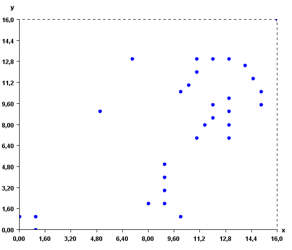
For example, the first instance is named "Instance1", and it is a vector with two values: 1 and 1 for the attributes X and Y, respectively.
This input file represents a set of 2D points. But note that, it is possible to use more than two attributes to describe instances. To give a better idea of what the input file looks like, here is a visual representation:
The distance function used by Optics is the Euclidian distance
What is the output?
DBScans groups vectors (points) in clusters based on density and distance between points.
Note that it is normal that DBScan may generate a cluster having less than minPts (this happens if the neibhoors of a core points get "stolen" by another cluster).
Note also that DBScan eliminate points that are seen as noise (a point having less than minPts neighboors within a radius of epsilon)
By running DBScan on the previous input file and minPts =2 and epsilon=2, we obtain the following output file containing 4 clusters:
@ATTRIBUTEDEF=X
@ATTRIBUTEDEF=Y
[Instance1 1.0 1.0][Instance3 1.0 0.0][Instance2 0.0 1.0]
[Instance14 10.0 1.0][Instance13 9.0 2.0][Instance28 9.0 3.0][Instance29 9.0 4.0][Instance12 8.0 2.0][Instance30 9.0 5.0]
[Instance27 10.0 10.5][Instance26 10.5 11.0][Instance4 11.0 12.0][Instance5 11.0 13.0][Instance21 12.0 13.0][Instance6 13.0 13.0][Instance21 14.0 12.5][Instance22 14.5 11.5][Instance23 15.0 10.5][Instance24 15.0 9.5]
[Instance11 11.0 7.0][Instance18 11.5 8.0][Instance7 12.0 8.5][Instance25 12.0 9.5][Instance8 13.0 8.0][Instance9 13.0 9.0][Instance10 13.0 7.0][Instance20 13.0 10.0]
The output file format is defined as follows. The first few lines indicate the attribute names. Each attribute is specified on a separated line with the keyword "ATTRIBUTEDEF=" followed by the attribute name (a string). Then, the list of clusters is indicated. Each cluster is specified on a separated line, listing the instances contained in the cluster. An instance is a name followed by a list of double values separated by " " and between the "[" and "]" characters.
The clusters found by the algorithm can be viewed visually using the "Cluster Viewer" provided in SPMF. If you are using the graphical interface of SPMF, click the checkbox "Cluster Viewer" before pressing the "Run Algorithm" button. The result will be displayed in the Cluster Viewer.
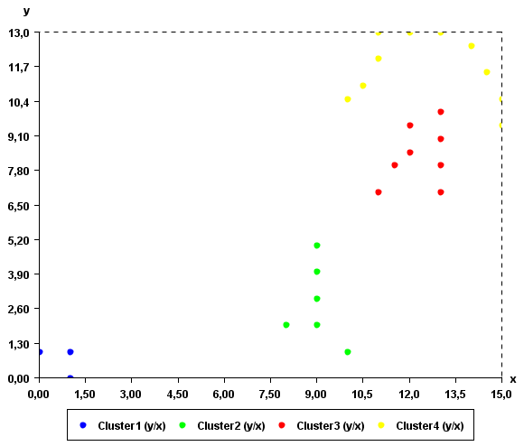
As it can be seen in this example, the result somewhat make sense. Points that are close to each other have put in the same clusters. An interesting thing about DBScan is that it can find clusters of various shapes.
Applying DBSCAN to time series
Note that the DBScan algorithm implementation in SPMF can also be applied to time series database such as the file contextSAX.txt in the SPMF distribution. To apply this algorithm to time series, it is necessary to set the "separator" parameter of this algorithm to "," since time series files separate values by "," instead of separating by spaces.
Where can I get more information about DBScan?
DBScan is a most famous data mining algorithm for clustering. It is described in almost all data mining books that focus on algorithms, and on many websites. The original article describing DBScan is:
Ester, Martin; Kriegel, Hans-Peter; Sander, Jörg; Xu, Xiaowei (1996). Simoudis, Evangelos; * Han, Jiawei; Fayyad, Usama M., eds. A density-based algorithm for discovering clusters in large spatial databases with noise. Proceedings of the Second International Conference on Knowledge Discovery and Data Mining (KDD-96). AAAI Press. pp. 226–231.