Calculate the second order differencing of time series (SPMF documentation)

This example explains how to calculate the second order differencing of time series using the SPMF open-source data mining library.

How to run this example?

• If you are using the graphical interface, (1) choose the "Calculate_second_order_differencing_of_time_series" algorithm, (2) select the input file "contextMovingAverage.txt", (3) set the separator to the comma ',' and then (4) click "Run algorithm".
• If you want to execute this example from the command line, then execute this command:
  java -jar spmf.jar run Calculate_second_order_differencing_of_time_series contextMovingAverage.txt output.txt ,
  in a folder containing spmf.jar and the example input file contextMovingAverage.txt.
• If you are using the source code version of SPMF, to run respectively this example, launch the file "MainTestSecondOrderDifferencingFileToFile.java"in the package ca.pfv.SPMF.tests.

What is the calculation of the second order differencing for time series?

Calculating the second order differencing of a time series is useful for converting a non stationary time series to a stationary form. It is calculated as follows. The i-th data point Y_i of a time series is replaced by Y'_i = Y_i - [2 * Y_(i-1)] + Y_(i-2).

What is the input of this algorithm?

The input is one or more time series. A time series is a sequence of floating-point decimal numbers (double values). A time-series can also have a name (a string).

Time series are used in many applications. An example of time series is the price of a stock on the stock market over time. Another example is a sequence of temperature readings collected using sensors.

For this example, consider the following time series:

Name	Data points
ECG1	3,2,8,9,8,9,8,7,6,7,5,4,2,7,9,8,5

This example time series database is provided in the file contextMovingAverage.txt of the SPMF distribution.

In SPMF, to read a time-series file, it is necessary to indicate the "separator", which is the character used to separate data points in the input file. In this example, the "separator" is the comma ',' symbol.

What is the output?

The output is the second order differencing of the time series received as input. It is calculated as follows. The i-th data point Y_i of a time series is replaced by Y'_i = Y_i - [2 * Y_(i-1)] + Y_(i-2).

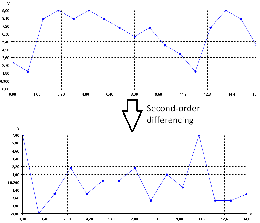
For example, in the above example, the result is:

Name	Data points
ECG1_SODIFF	7.0,-5.0,-2.0,2.0,-2.0,0.0,0.0,2.0,-3.0,1.0,-1.0,7.0,-3.0,-3.0,-2.0

To see the result visually, it is possible to use the SPMF time series viewer, described in another example of this documentation. In the following figure, the original time series is displayed (top) and its second order differencing (bottom).

Input file format

The input file format is defined as follows. It is a text file. The text file contains one or more time series. Each time series is represented by two lines in the input file. The second line contains the string "@NAME=" followed by the name of the time series. The second line is a list of data points, where data points are floating-point decimal numbers separated by a separator character (here the ',' symbol).

For example, the input file of the previous example, named contextMovingAverage.txt is defined as follows:

@NAME=ECG2
3,2,8,9,8,9,8,7,6,7,5,4,2,7,9,8,5

Consider the second two lines. It indicates that the second time series name is "ECG2" and that it consits of the data points: 3,2,8,9,8,9,8,7,6,7,5,4,2,7,9,8, and 5. Then, three other time series are provided in the same file, which follows the same format.

But note that it is possible to have more than one time series per file. For example, this is another input file called contextSax.txt, which contains 4 time series.

@NAME=ECG1
1,2,3,4,5,6,7,8,9,10
@NAME=ECG2
1.5,2.5,10,9,8,7,6,5
@NAME=ECG3
-1,-2,-3,-4,-5
@NAME=ECG4
-2.0,-3.0,-4.0,-5.0,-6.0

Output file format

The output file format is the same as the input format. For example, there is the result of this example:

@NAME=ECG2_SODIFF
7.0,-5.0,-2.0,2.0,-2.0,0.0,0.0,2.0,-3.0,1.0,-1.0,7.0,-3.0,-3.0,-2.0

Implementation details

Beside the second order differencing, SPMF also offers first-order differencing and various other operations for time series.

Where can I get more information about the second order differencing?

The second order differencing is a basic operation for analyzing time series. It is described in many websites and books.