Documentation
This section provides examples of how to use SPMF
to perform various data mining tasks.
If you have any question or if you want to report a bug,
you can check the FAQ,
post in the forum
or contact me.
You can also have a look at the various articles that I have referenced
on the algorithms
page of this website to learn more about each algorithm.
List of examples
Itemset Mining (Frequent Itemsets, Rare
Itemsets, etc.)
High-Utility Pattern Mining
Association Rule Mining
Clustering
Sequential Pattern Mining
Sequential Rule Mining
Sequence Prediction (source code version only)
Periodic pattern mining
Text Mining
Time Series Mining
Classification
Tools
Example 1 : Mining Frequent Itemsets by Using the Apriori
Algorithm
How to run this example?
- If you are using the graphical interface, (1)
choose the "Apriori"
algorithm, (2) select the input file "contextPasquier99.txt", (3) set the
output file name (e.g. "output.txt") (4)
set minsup to 40% and (5) click "Run algorithm".
- If you want to execute this example from the command line,
then execute this command:
java -jar spmf.jar run Apriori
contextPasquier99.txt output.txt 40% in a folder containing spmf.jar and the example input file contextPasquier99.txt.
- If you are using the source code version of SPMF, launch
the file "MainTestApriori_saveToMemory.java"
in the package ca.pfv.SPMF.tests.
What is Apriori?
Apriori is an algorithm for discovering frequent
itemsets in transaction databases. It was proposed by Agrawal &
Srikant (1993).
What is the input of the Apriori algorithm?
The input is a transaction database (aka binary
context) and a threshold named minsup (a
value between 0 and 100 %).
A transaction database is a set of transactions.
Each transaction is a set of items. For example,
consider the following transaction database. It contains 5 transactions
(t1, t2, ..., t5) and 5 items (1,2, 3, 4, 5). For example, the first
transaction represents the set of items 1, 3 and 4. This database is
provided as the file contextPasquier99.txt in the
SPMF distribution. It is important to note that an item is not allowed
to appear twice in the same transaction and that items are assumed to
be sorted by lexicographical order in a transaction.
| Transaction id |
Items |
| t1 |
{1, 3, 4} |
| t2 |
{2, 3, 5} |
| t3 |
{1, 2, 3, 5} |
| t4 |
{2, 5} |
| t5 |
{1, 2, 3, 5} |
What is the output of the Apriori algorithm?
Apriori is an algorithm for discovering itemsets (group of items)
occurring frequently in a transaction database (frequent
itemsets). A frequent itemset is an itemset appearing in at
least minsup transactions from the transaction database,
where minsup is a parameter given by the user.
For example, if Apriori is run on the previous
transaction database with a minsup of 40 % (2 transactions), Apriori
produces the following result:
| itemsets |
support |
| {1} |
3 |
| {2} |
4 |
| {3} |
4 |
| {5} |
4 |
| {1, 2} |
2 |
| {1, 3} |
3 |
| {1, 5} |
2 |
| {2, 3} |
3 |
| {2, 5} |
4 |
| {3, 5} |
3 |
| {1, 2, 3} |
2 |
| {1, 2, 5} |
2 |
| {1, 3, 5} |
2 |
| {2, 3, 5} |
3 |
| {1, 2, 3, 5} |
2 |
How should I interpret the results?
In the results, each itemset is annotated with its
support. The support of an itemset is how many times
the itemset appears in the transaction database. For example, the
itemset {2, 3 5} has a support of 3 because it appears in transactions
t2, t3 and t5. It is a frequent itemset because its support is higher
or equal to the minsup parameter.
Input file format
The input file format for Apriori is defined as
follows. It is a text file. An item is represented by a positive
integer. A transaction is a line in the text file. In each line
(transaction), items are separated by a single space. It is assumed
that all items within a same transaction (line) are sorted according to
a total order (e.g. ascending order) and that no item can appear twice
within the same line.
For example, for the previous example, the input file is defined
as follows:
1 3 4
2 3 5
1 2 3 5
2 5
1 2 3 5
Note that it is also possible to use the ARFF format
as an alternative to the default input format. The specification of the
ARFF format can be found here.
Most features of the ARFF format are supported except that (1) the
character "=" is forbidden and (2) escape characters are not
considered. Note that when the ARFF format is used, the performance of
the data mining algorithms will be slightly less than if the native
SPMF file format is used because a conversion of the input file will be
automatically performed before launching the algorithm and the result
will also have to be converted. This cost however should be small.
Output file format
The output file format is defined as follows. It
is a text file, where each line represents a frequent itemset. On each
line, the items of the itemset are first listed. Each item is
represented by an integer and it is followed by a single space. After,
all the items, the keyword "#SUP:" appears, which is followed by an
integer indicating the support of the itemset, expressed as a number of
transactions. For example, here is the output file for this example.
The first line indicates the frequent itemset consisting of the item 1
and it indicates that this itemset has a support of 3 transactions.
1 #SUP: 3
2 #SUP: 4
3 #SUP: 4
5 #SUP: 4
1 2 #SUP: 2
1 3 #SUP: 3
1 5 #SUP: 2
2 3 #SUP: 3
2 5 #SUP: 4
3 5 #SUP: 3
1 2 3 #SUP: 2
1 2 5 #SUP: 2
1 3 5 #SUP: 2
2 3 5 #SUP: 3
1 2 3 5 #SUP: 2
Note that if the ARFF format is used as input instead of the
default input format, the output format will be the same except that
items will be represented by strings instead of integers.
Performance
The Apriori algorithm is an important algorithm for historical
reasons and also because it is a simple algorithm that is easy to
learn. However, faster and more memory efficient algorithms have been
proposed. If efficiency is required, it is recommended to use a more
efficient algorithm like FPGrowth instead of Apriori. You can see a
performance comparison of Apriori, FPGrowth, and other frequent itemset
mining algorithms by clicking on the "performance"
section of this website.
Implementation details
In SPMF, there is also an implementation of Apriori that uses a
hash-tree as an internal structure to store candidates. This
structure provide a more efficient way to count the support of
itemsets. This version of Apriori is named "Apriori_with_hash_tree"
in the GUI of SPMF and the command line. For the source code version,
it can be run by executing the test file MainTestAprioriHT_saveToFile.java.
This version of Apriori can be up to twice faster than the regular
version in some cases but it uses more memory. This version of Apriori
has two parameters: (1) minsup and (2) the number of child nodes that
each node in the hash-tree should have. For the second parameter, we
suggest to use the value 30.
Where can I get more information about the Apriori algorithm?
This is the technical report published in 1994 describing
Apriori.
R. Agrawal and R. Srikant. Fast algorithms for mining association rules in large
databases. Research Report RJ 9839, IBM Almaden Research Center,
San Jose, California, June 1994.
You can also read chapter 6
of the book "introduction to data mining" which provide a nice and
easy to understand introduction to Apriori.
Example 2 : Mining Frequent
Itemsets by Using the AprioriTid Algorithm
How to run this example?
- If you are using the graphical interface, (1)
choose the "Apriori_TID"
algorithm , (2) select the input file "contextPasquier99.txt", (3) set the
output file name (e.g. "output.txt") (4)
set minsup to 40% and (5) click "Run algorithm".
- If you want to execute this example from the command line,
then execute this command:
java -jar spmf.jar run Apriori_TID
contextPasquier99.txt output.txt 40% in a folder containing spmf.jar and the example input file contextPasquier99.txt.
- If you are using the source code version of SPMF, launch
the file "MainTestAprioriTID_saveToFile.java"
in the package ca.pfv.SPMF.tests.
What is AprioriTID?
AprioriTID is an algorithm for discovering frequent itemsets
(groups of items appearing frequently) in a transaction database. It
was proposed by Agrawal & Srikant (1993).
AprioriTID is a variation of the Apriori algorithm. It was
proposed in the same article as Apriori as an alternative
implementation of Apriori. It produces the same output as Apriori. But
it uses a different mechanism for counting the support of itemsets.
What is the input of the AprioriTID algorithm?
The input is a transaction database (aka
binary context) and a threshold named minsup
(a value between 0 and 100 %).
A transaction database is a set of
transactions. Each transaction is a set of items. For
example, consider the following transaction database. It contains 5
transactions (t1, t2, ..., t5) and 5 items (1,2, 3, 4, 5). For example,
the first transaction represents the set of items 1, 3 and 4. This
database is provided as the file contextPasquier99.txt
in the SPMF distribution. It is important to note that an item is not
allowed to appear twice in the same transaction and that items are
assumed to be sorted by lexicographical order in a transaction.
| Transaction id |
Items |
| t1 |
{1, 3, 4} |
| t2 |
{2, 3, 5} |
| t3 |
{1, 2, 3, 5} |
| t4 |
{2, 5} |
| t5 |
{1, 2, 3, 5} |
What is the output of the AprioriTID algorithm?
AprioriTID is an algorithm for discovering
itemsets (group of items) occurring frequently in a transaction
database (frequent itemsets). A frequent itemset is an
itemset appearing in at least minsup transactions from the
transaction database, where minsup is a parameter given by
the user.
For example, if AprioriTID is run on the
previous transaction database with a minsup of 40 % (2 transactions), AprioriTID
produces the following result:
| itemsets |
support |
| {1} |
3 |
| {2} |
4 |
| {3} |
4 |
| {5} |
4 |
| {1, 2} |
2 |
| {1, 3} |
3 |
| {1, 5} |
2 |
| {2, 3} |
3 |
| {2, 5} |
4 |
| {3, 5} |
3 |
| {1, 2, 3} |
2 |
| {1, 2, 5} |
2 |
| {1, 3, 5} |
2 |
| {2, 3, 5} |
3 |
| {1, 2, 3, 5} |
2 |
How should I interpret the results?
In the results, each itemset is annotated with its support. The support
of an itemset is how many times the itemset appears in the transaction
database. For example, the itemset {2, 3 5} has a support of 3 because
it appears in transactions t2, t3 and t5. It is a frequent itemset
because its support is higher or equal to the minsup parameter.
Input file format
The input file format used by AprioriTID is
defined as follows. It is a text file. An item is represented by a
positive integer. A transaction is a line in the text file. In each
line (transaction), items are separated by a single space. It is
assumed that all items within a same transaction (line) are sorted
according to a total order (e.g. ascending order) and that no item can
appear twice within the same line.
For example, for the previous example, the input file is defined
as follows:
1 3 4
2 3 5
1 2 3 5
2 5
1 2 3 5
Note that it is also possible to use the ARFF format
as an alternative to the default input format. The specification of the
ARFF format can be found here.
Most features of the ARFF format are supported except that (1) the
character "=" is forbidden and (2) escape characters are not
considered. Note that when the ARFF format is used, the performance of
the data mining algorithms will be slightly less than if the native
SPMF file format is used because a conversion of the input file will be
automatically performed before launching the algorithm and the result
will also have to be converted. This cost however should be small.
Output file format
The output file format is defined as follows. It
is a text file, where each line represents a frequent itemset. On each
line, the items of the itemset are first listed. Each item is
represented by an integer and it is followed by a single space. After,
all the items, the keyword "#SUP:" appears, which is followed by an
integer indicating the support of the itemset, expressed as a number of
transactions. For example, here is the output file for this example.
The first line indicates the frequent itemset consisting of the item 1
and it indicates that this itemset has a support of 3 transactions.
1 #SUP: 3
2 #SUP: 4
3 #SUP: 4
5 #SUP: 4
1 2 #SUP: 2
1 3 #SUP: 3
1 5 #SUP: 2
2 3 #SUP: 3
2 5 #SUP: 4
3 5 #SUP: 3
1 2 3 #SUP: 2
1 2 5 #SUP: 2
1 3 5 #SUP: 2
2 3 5 #SUP: 3
1 2 3 5 #SUP: 2
Note that if the ARFF format is used as input instead of the
default input format, the output format will be the same except that
items will be represented by strings instead of integers.
Performance
The Apriori and AprioriTID algorithms are important algorithms for
historical reasons and also because they are simple algorithms that are
easy to learn. However, faster and more memory efficient algorithms
have been proposed. For efficiency, it is recommended to use more
efficient algorithms like FPGrowth instead of
AprioriTID or Apriori. You can see a performance comparison of Apriori,
AprioriTID, FPGrowth, and other frequent itemset mining algorithms by
clicking on the "performance"
section of this website.
Implementation details
There are two
versions of AprioriTID in SPMF. The first one is
called AprioriTID and is the regular AprioriTID
algorithm. The second one is called AprioriTID_Bitset
and uses bitsets as internal structures
instead of HashSet of Integers to represent sets of transactions IDs.
The advantage of the bitset version is that using bitsets for
representing sets of transactions IDs is more memory efficient and
performing the intersection of two sets of transactions IDs is more
efficient with bitsets (it is done by doing the logical AND operation).
Optional parameter(s)
This implementation allows to specify
additional optional parameter(s) :
- "show transaction ids?" (true/false) This parameter allows to
specify that transaction ids of transactions containing a pattern should be
output for each pattern found. For example, if the parameter is set to
true, each pattern in the output file will be followed by the keyword
#TID followed by a list of transaction ids (integers separated by space).
For example, a line terminated by "#TID: 0 2" means that the pattern on
this line appears in the first and the third transactions of the transaction
database (transactions with ids 0 and 2).
These parameter(s) are available in the GUI of SPMF and also in
the example(s) "MainTestAprioriTID_..._saveToFile
.java" provided in the source code of SPMF.
The parameter(s) can be also used in the command line with the Jar
file. If you want to use these optional parameter(s) in the command
line, it can be done as follows. Consider this example:
java -jar spmf.jar run Apriori_TID
contextPasquier99.txt output.txt 40% true
This command means to apply the algorithm on the file
"contextPasquier99.txt" and output the results to "output.txt".
Moreover, it specifies that the user wants to find patterns for minsup = 40%, and that transaction
ids should be output for each pattern found.
Where can I get more information about the AprioriTID algorithm?
This is the technical report published in 1994 describing
Apriori and AprioriTID.
R. Agrawal and R. Srikant. Fast algorithms for mining association rules in large
databases. Research Report RJ 9839, IBM Almaden Research Center,
San Jose, California, June 1994.
You can also read chapter 6
of the book "introduction to data mining" which provide a nice and
easy to understand introduction to Apriori.
Example 3 : Mining Frequent Itemsets by Using the FP-Growth
Algorithm
How to run this example?
- If you are using the graphical interface, (1)
choose the "FPGrowth_itemsets"
algorithm, (2) select the input file "contextPasquier99.txt", (3) set the
output file name (e.g. "output.txt") (4)
set minsup to 40% and (5) click "Run algorithm".
- If you want to execute this example from the command line,
then execute this command:
java -jar spmf.jar run FPGrowth_itemsets contextPasquier99.txt
output.txt 40% in a folder containing spmf.jar
and the example input file contextPasquier99.txt.
- If you are using the source code version of SPMF, launch
the file "MainTestFPGrowth_saveToFile.java"
in the package ca.pfv.SPMF.tests.
What is FPGrowth?
FPGrowth is an algorithm for discovering frequent itemsets in a
transaction database. It was proposed by Han et al. (2000). FPGrowth is
a very fast and memory efficient algorithm. It uses a special internal
structure called an FP-Tree.
What is the input of the FPGrowth algorithm?
The input of FPGrowth is a transaction
database (aka binary context) and a threshold named minsup
(a value between 0 and 100 %).
A transaction database is a set of
transactions. Each transaction is a set of items. For
example, consider the following transaction database. It contains 5
transactions (t1, t2, ..., t5) and 5 items (1,2, 3, 4, 5). For example,
the first transaction represents the set of items 1, 3 and 4. This
database is provided as the file contextPasquier99.txt
in the SPMF distribution. It is important to note that an item is not
allowed to appear twice in the same transaction and that items are
assumed to be sorted by lexicographical order in a transaction.
| Transaction id |
Items |
| t1 |
{1, 3, 4} |
| t2 |
{2, 3, 5} |
| t3 |
{1, 2, 3, 5} |
| t4 |
{2, 5} |
| t5 |
{1, 2, 3, 5} |
What is the output of the FPGrowth algorithm?
FPGrowth is an algorithm for discovering itemsets
(group of items) occurring frequently in a transaction database (frequent
itemsets). A frequent itemset is an itemset appearing in at
least minsup transactions from the transaction database,
where minsup is a parameter given by the user.
For example, if FPGrowth is run on the previous
transaction database with a minsup of 40 % (2 transactions),
FPGrowth produces the following result:
| itemsets |
support |
| {1} |
3 |
| {2} |
4 |
| {3} |
4 |
| {5} |
4 |
| {1, 2} |
2 |
| {1, 3} |
3 |
| {1, 5} |
2 |
| {2, 3} |
3 |
| {2, 5} |
4 |
| {3, 5} |
3 |
| {1, 2, 3} |
2 |
| {1, 2, 5} |
2 |
| {1, 3, 5} |
2 |
| {2, 3, 5} |
3 |
| {1, 2, 3, 5} |
2 |
How should I interpret the results?
In the results, each itemset is annotated with its
support. The support of an itemset is how many times
the itemset appears in the transaction database. For example, the
itemset {2, 3 5} has a support of 3 because it appears in transactions
t2, t3 and t5. It is a frequent itemset because its support is higher
or equal to the minsup parameter.
Input file format
The input file format used by FPGrowth is
defined as follows. It is a text file. An item is represented by a
positive integer. A transaction is a line in the text file. In each
line (transaction), items are separated by a single space. It is
assumed that all items within a same transaction (line) are sorted
according to a total order (e.g. ascending order) and that no item can
appear twice within the same line.
For example, for the previous example, the input file is defined
as follows:
1 3 4
2 3 5
1 2 3 5
2 5
1 2 3 5
Note that it is also possible to use the ARFF format
as an alternative to the default input format. The specification of the
ARFF format can be found here.
Most features of the ARFF format are supported except that (1) the
character "=" is forbidden and (2) escape characters are not
considered. Note that when the ARFF format is used, the performance of
the data mining algorithms will be slightly less than if the native
SPMF file format is used because a conversion of the input file will be
automatically performed before launching the algorithm and the result
will also have to be converted. This cost however should be small.
Output file format
The output file format is defined as follows. It
is a text file, where each line represents a frequent itemset. On each
line, the items of the itemset are first listed. Each item is
represented by an integer and it is followed by a single space. After,
all the items, the keyword "#SUP:" appears, which is followed by an
integer indicating the support of the itemset, expressed as a number of
transactions. For example, here is the output file for this example.
The first line indicates the frequent itemset consisting of the item 1
and it indicates that this itemset has a support of 3 transactions.
1 #SUP: 3
2 #SUP: 4
3 #SUP: 4
5 #SUP: 4
1 2 #SUP: 2
1 3 #SUP: 3
1 5 #SUP: 2
2 3 #SUP: 3
2 5 #SUP: 4
3 5 #SUP: 3
1 2 3 #SUP: 2
1 2 5 #SUP: 2
1 3 5 #SUP: 2
2 3 5 #SUP: 3
1 2 3 5 #SUP: 2
Note that if the ARFF format is used as input instead of the
default input format, the output format will be the same except that
items will be represented by strings instead of integers.
Performance
There exists several algorithms for mining frequent itemsets. In
SPMF, you can try for example Apriori, AprioriTID, Eclat, HMine, Relim
and more. Among all these algorithms, FPGrowth is
generally the fastest and most memory efficient algorithm. You can see
a performance comparison by clicking on the "performance"
section of this website.
Where can I get more information about the FPGrowth algorithm?
This is the journal article describing FPGrowth:
Jiawei Han, Jian Pei, Yiwen Yin, Runying Mao: Mining
Frequent Patterns without Candidate Generation: A Frequent-Pattern Tree
Approach. Data Min. Knowl. Discov. 8(1): 53-87 (2004)
You can also read chapter 6
of the book "introduction to data mining" which provide an easy to
understand introduction to FPGrowth (but does not give all the details).
Example 4 : Mining Frequent Itemsets by Using the Relim
Algorithm
How to run this example?
- If you are using the graphical interface, (1)
choose the "Relim"
algorithm, (2) select the input file "contextPasquier99.txt", (3) set the
output file name (e.g. "output.txt") (4)
set minsup to 40% and (5) click "Run algorithm".
- If you want to execute this example from the command line,
then execute this command:
java -jar spmf.jar run Relim contextPasquier99.txt
output.txt 40% in a folder containing spmf.jar
and the example input file contextPasquier99.txt.
- If you are using the source code version of SPMF, launch
the file "MainTestRelim.java"
in the package ca.pfv.SPMF.tests.
What is Relim?
Relim is an algorithm for discovering frequent
itemsets in a transaction database. Relim was proposed by Borgelt
(2005). It is not a very efficient algorithm. It is included in SPMF
for comparison purposes.
What is the input of the Relim algorithm?
The input is a transaction database (aka binary
context) and a threshold named minsup (a
value between 0 and 100 %).
A transaction database is a set of transactions.
Each transaction is a set of items. For example,
consider the following transaction database. It contains 5 transactions
(t1, t2, ..., t5) and 5 items (1,2, 3, 4, 5). For example, the first
transaction represents the set of items 1, 3 and 4. This database is
provided as the file contextPasquier99.txt in the
SPMF distribution. It is important to note that an item is not allowed
to appear twice in the same transaction and that items are assumed to
be sorted by lexicographical order in a transaction.
| Transaction id |
Items |
| t1 |
{1, 3, 4} |
| t2 |
{2, 3, 5} |
| t3 |
{1, 2, 3, 5} |
| t4 |
{2, 5} |
| t5 |
{1, 2, 3, 5} |
What is the output of the Relim algorithm?
Relim is an algorithm for discovering itemsets
(group of items) occurring frequently in a transaction database (frequent
itemsets). A frequent itemset is an itemset appearing in at
least minsup transactions from the transaction database,
where minsup is a parameter given by the user.
For example, if Relim is run on the previous
transaction database with a minsup of 40 % (2 transactions),
Relim produces the following result:
| itemsets |
support |
| {1} |
3 |
| {2} |
4 |
| {3} |
4 |
| {5} |
4 |
| {1, 2} |
2 |
| {1, 3} |
3 |
| {1, 5} |
2 |
| {2, 3} |
3 |
| {2, 5} |
4 |
| {3, 5} |
3 |
| {1, 2, 3} |
2 |
| {1, 2, 5} |
2 |
| {1, 3, 5} |
2 |
| {2, 3, 5} |
3 |
| {1, 2, 3, 5} |
2 |
How should I interpret the results?
In the results, each itemset is annotated with its support. The support
of an itemset is how many times the itemset appears in the transaction
database. For example, the itemset {2, 3 5} has a support of 3 because
it appears in transactions t2, t3 and t5. It is a frequent itemset
because its support is higher or equal to the minsup parameter.
Input file format
The input file format used by Relim is defined
as follows. It is a text file. An item is represented by a positive
integer. A transaction is a line in the text file. In each line
(transaction), items are separated by a single space. It is assumed
that all items within a same transaction (line) are sorted according to
a total order (e.g. ascending order) and that no item can appear twice
within the same line.
For example, for the previous example, the input file is defined
as follows:
1 3 4
2 3 5
1 2 3 5
2 5
1 2 3 5
Note that it is also possible to use the ARFF format
as an alternative to the default input format. The specification of the
ARFF format can be found here.
Most features of the ARFF format are supported except that (1) the
character "=" is forbidden and (2) escape characters are not
considered. Note that when the ARFF format is used, the performance of
the data mining algorithms will be slightly less than if the native
SPMF file format is used because a conversion of the input file will be
automatically performed before launching the algorithm and the result
will also have to be converted. This cost however should be small.
Output file format
The output file format is defined as follows. It
is a text file, where each line represents a frequent itemset. On each
line, the items of the itemset are first listed. Each item is
represented by an integer and it is followed by a single space. After,
all the items, the keyword "#SUP:" appears, which is followed by an
integer indicating the support of the itemset, expressed as a number of
transactions. For example, here is the output file for this example.
The first line indicates the frequent itemset consisting of the item 1
and it indicates that this itemset has a support of 3 transactions.
1 #SUP: 3
2 #SUP: 4
3 #SUP: 4
5 #SUP: 4
1 2 #SUP: 2
1 3 #SUP: 3
1 5 #SUP: 2
2 3 #SUP: 3
2 5 #SUP: 4
3 5 #SUP: 3
1 2 3 #SUP: 2
1 2 5 #SUP: 2
1 3 5 #SUP: 2
2 3 5 #SUP: 3
1 2 3 5 #SUP: 2
Note that if the ARFF format is used as input instead of the
default input format, the output format will be the same except that
items will be represented by strings instead of integers.
Performance
There exists several algorithms for mining frequent itemsets.
Relim is not a very efficient algorithm. For efficiency, it is
recommended to use FPGrowth for better performance. You can see a
performance comparison by clicking on the "performance"
section of this website.
Where can I get more information about the FPGrowth algorithm?
This is the conference article describing Relim:
Keeping
Things Simple: Finding Frequent Item Sets by Recursive Elimination Christian
Borgelt. Workshop Open Source Data Mining Software (OSDM'05, Chicago,
IL), 66-70. ACM Press, New York, NY, USA 2005
Note that the author of Relim and collaborators have proposed
extensions and additional optimizations of Relim that I have not
implemented.
Example 5 : Mining Frequent Itemsets by Using the Eclat /
dEclat Algorithm
How to run this example?
- If you are using the graphical interface, (1)
choose the "Eclat" or "dEclat" algorithm,
(2) select the input file "contextPasquier99.txt",
(3) set the output file name (e.g. "output.txt")
(4) set minsup to 40% and (5) click "Run algorithm".
- If you want to execute this example from the command line,
then execute this command:
java -jar spmf.jar run Eclat
contextPasquier99.txt output.txt 40% in a folder containing spmf.jar and the example input file contextPasquier99.txt.
- If you are using the source code version of SPMF, to
run respectively Eclat or dEclat, launch
the file "MainTestEclat_saveToMemory.java"
or "MainTestDEclat_bitset_saveToMemory.java"in
the package ca.pfv.SPMF.tests.
What is Eclat ?
Eclat is an algorithm for discovering frequent
itemsets in a transaction database. It was proposed by Zaki (2001).
Contrarily to algorithms such as Apriori, Eclat uses
a depth-first search for discovering frequent itemsets instead of a
breath-first search.
dEclat is a variation of the Eclat algorithm
that is implemented using a structure called "diffsets" rather than
"tidsets".
What is the input of the Eclat algorithm?
The input is a transaction database (aka
binary context) and a threshold named minsup
(a value between 0 and 100 %).
A transaction database is a set of
transactions. Each transaction is a set of items. For
example, consider the following transaction database. It contains 5
transactions (t1, t2, ..., t5) and 5 items (1,2, 3, 4, 5). For example,
the first transaction represents the set of items 1, 3 and 4. This
database is provided as the file contextPasquier99.txt
in the SPMF distribution. It is important to note that an item is not
allowed to appear twice in the same transaction and that items are
assumed to be sorted by lexicographical order in a transaction.
| Transaction id |
Items |
| t1 |
{1, 3, 4} |
| t2 |
{2, 3, 5} |
| t3 |
{1, 2, 3, 5} |
| t4 |
{2, 5} |
| t5 |
{1, 2, 3, 5} |
What is the output of the Eclat algorithm?
Eclat is an algorithm for discovering itemsets
(group of items) occurring frequently in a transaction database (frequent
itemsets). A frequent itemset is an itemset appearing in at
least minsup transactions from the transaction database,
where minsup is a parameter given by the user.
For example, if Eclat is run on the previous
transaction database with a minsup of 40 % (2 transactions),
Eclat produces the following result:
| itemsets |
support |
| {1} |
3 |
| {2} |
4 |
| {3} |
4 |
| {5} |
4 |
| {1, 2} |
2 |
| {1, 3} |
3 |
| {1, 5} |
2 |
| {2, 3} |
3 |
| {2, 5} |
4 |
| {3, 5} |
3 |
| {1, 2, 3} |
2 |
| {1, 2, 5} |
2 |
| {1, 3, 5} |
2 |
| {2, 3, 5} |
3 |
| {1, 2, 3, 5} |
2 |
How should I interpret the results?
Each frequent itemset is annotated with its support. The support
of an itemset is how many times the itemset appears in the transaction
database. For example, the itemset {2, 3 5} has a support of 3 because
it appears in transactions t2, t3 and t5. It is a frequent itemset
because its support is higher or equal to the minsup parameter.
Input file format
The input file format used by ECLAT is defined
as follows. It is a text file. An item is represented by a positive
integer. A transaction is a line in the text file. In each line
(transaction), items are separated by a single space. It is assumed
that all items within a same transaction (line) are sorted according to
a total order (e.g. ascending order) and that no item can appear twice
within the same line.
For example, for the previous example, the input file is defined
as follows:
1 3 4
2 3 5
1 2 3 5
2 5
1 2 3 5
Note that it is also possible to use the ARFF format
as an alternative to the default input format. The specification of the
ARFF format can be found here.
Most features of the ARFF format are supported except that (1) the
character "=" is forbidden and (2) escape characters are not
considered. Note that when the ARFF format is used, the performance of
the data mining algorithms will be slightly less than if the native
SPMF file format is used because a conversion of the input file will be
automatically performed before launching the algorithm and the result
will also have to be converted. This cost however should be small.
Output file format
The output file format is defined as follows. It
is a text file, where each line represents a frequent itemset. On each
line, the items of the itemset are first listed. Each item is
represented by an integer and it is followed by a single space. After,
all the items, the keyword "#SUP:" appears, which is followed by an
integer indicating the support of the itemset, expressed as a number of
transactions. For example, here is the output file for this example.
The first line indicates the frequent itemset consisting of the item 1
and it indicates that this itemset has a support of 3 transactions.
1 #SUP: 3
2 #SUP: 4
3 #SUP: 4
5 #SUP: 4
1 2 #SUP: 2
1 3 #SUP: 3
1 5 #SUP: 2
2 3 #SUP: 3
2 5 #SUP: 4
3 5 #SUP: 3
1 2 3 #SUP: 2
1 2 5 #SUP: 2
1 3 5 #SUP: 2
2 3 5 #SUP: 3
1 2 3 5 #SUP: 2
Note that if the ARFF format is used as input instead of the
default input format, the output format will be the same except that
items will be represented by strings instead of integers.
Performance
There exists several algorithms for mining frequent itemsets.
Eclat is one of the best. But generally, FPGrowth is a better
algorithm. You can see a performance comparison by clicking on the "performance"
section of this website. Note that recently (SPMF v0.96e), the Eclat
implementation was optimized and is sometimes faster than FPGrowth.
Nevertheless, the Eclat algorithm is interesting because it uses a
depth-first search. For some extensions of the problem of itemset
mining such as mining high utility itemsets (see the HUI-Miner
algorithm), the search procedure of Eclat works very well.
Implementation details
In SPMF, there are four versions of ECLAT. The first one is named "Eclat" and uses HashSets of Integers for
representing sets of transaction IDs (tidsets). The second version is
named "Eclat_bitset" and uses bitsets for
representing tidsets. Using bitsets has the advantage of generally
being more memory efficient and can also make the algorithm faster
depending on the dataset.
There is also two versions of dEclat, which
utilizes a structure called diffsets instead of tidsets. The versions
having diffsets implemented as HashSets of integers and the version
having diffsets implemented as bitsets are respectively named "dEclat_bitset" and "dEclat"
Optional parameter(s)
This implementation allows to specify
additional optional parameter(s) :
- "show transaction ids?" (true/false) This parameter allows to
specify that transaction ids of transactions containing a pattern should be
output for each pattern found. For example, if the parameter is set to
true, each pattern in the output file will be followed by the keyword
#TID followed by a list of transaction ids (integers separated by space).
For example, a line terminated by "#TID: 0 2" means that the pattern on
this line appears in the first and the third transactions of the transaction
database (transactions with ids 0 and 2).
These parameter(s) are available in the GUI of SPMF and also in
the example(s) "MainTestEclat_..._saveToFile
.java" provided in the source code of SPMF.
The parameter(s) can be also used in the command line with the Jar
file. If you want to use these optional parameter(s) in the command
line, it can be done as follows. Consider this example:
java -jar spmf.jar run Eclat
contextPasquier99.txt output.txt 40% true
This command means to apply the algorithm on the file
"contextPasquier99.txt" and output the results to "output.txt".
Moreover, it specifies that the user wants to find patterns for minsup = 40%, and that transaction
ids should be output for each pattern found.
Where can I get more information about the Eclat algorithm?
Here is an article describing the Eclat algorithm:
Mohammed Javeed Zaki: Scalable
Algorithms for Association Mining. IEEE Trans. Knowl. Data Eng.
12(3): 372-390 (2000)
Here is an article describing the dEclat variation:
Zaki, M.J., Gouda, K.: Fast vertical mining using diffsets. Technical
Report 01-1, Computer Science Dept., Rensselaer Polytechnic Institute
(March 2001) 10
Example 6 : Mining Frequent Itemsets by Using the HMine
Algorithm
How to run this example?
- If you are using the graphical interface, (1)
choose the "HMine"
algorithm, (2) select the input file "contextPasquier99.txt", (3) set the
output file name (e.g. "output.txt") (4)
set minsup to 0.4 and (5) click "Run algorithm".
- If you want to execute this example from the command line,
then execute this command:
java -jar spmf.jar run HMine contextPasquier99.txt output.txt
0.4 in a folder containing spmf.jar
and the example input file contextPasquier99.txt.
- If you are using the source code version of SPMF, launch
the file "MainTestHMine.java"
in the package ca.pfv.SPMF.tests.
What is H-Mine ?
H-Mine is an algorithm for discovering frequent itemsets in
transaction databases, proposed by Pei et al. (2001). Contrarily to
previous algorithms such as Apriori, H-Mine uses a pattern-growth
approach to discover frequent itemsets.
What is the input of the H-Mine algorithm?
The input of H-Mine is a transaction database
(aka binary context) and a threshold named minsup
(a value between 0 and 100 %).
A transaction database is a set of transactions.
Each transaction is a set of items. For example,
consider the following transaction database. It contains 5 transactions
(t1, t2, ..., t5) and 5 items (1,2, 3, 4, 5). For example, the first
transaction represents the set of items 1, 3 and 4. This database is
provided as the file contextPasquier99.txt in the
SPMF distribution. It is important to note that an item is not allowed
to appear twice in the same transaction and that items are assumed to
be sorted by lexicographical order in a transaction.
| Transaction id |
Items |
| t1 |
{1, 3, 4} |
| t2 |
{2, 3, 5} |
| t3 |
{1, 2, 3, 5} |
| t4 |
{2, 5} |
| t5 |
{1, 2, 3, 5} |
What is the output of the H-Mine algorithm?
H-Mine is an algorithm for discovering itemsets
(group of items) occurring frequently in a transaction database (frequent
itemsets). A frequent itemset is an itemset appearing in at
least minsup transactions from the transaction database,
where minsup is a parameter given by the user.
For example, if H-Mine is run on the previous
transaction database with a minsup of 40 % (2 transactions),
H-Mine produces the following result:
| itemsets |
support |
| {1} |
3 |
| {2} |
4 |
| {3} |
4 |
| {5} |
4 |
| {1, 2} |
2 |
| {1, 3} |
3 |
| {1, 5} |
2 |
| {2, 3} |
3 |
| {2, 5} |
4 |
| {3, 5} |
3 |
| {1, 2, 3} |
2 |
| {1, 2, 5} |
2 |
| {1, 3, 5} |
2 |
| {2, 3, 5} |
3 |
| {1, 2, 3, 5} |
2 |
How should I interpret the results?
In the results, each itemset is annotated with its
support. The support of an itemset is how many times
the itemset appears in the transaction database. For example, the
itemset {2, 3 5} has a support of 3 because it appears in transactions
t2, t3 and t5. It is a frequent itemset because its support is higher
or equal to the minsup parameter.
Performance
There exists several algorithms for mining frequent itemsets.
H-Mine is claimed to be one of the best by their author. The
implementation offered in SPMF is well-optimized.
Input file format
The input file format used by H-Mine is defined
as follows. It is a text file. An item is represented by a positive
integer. A transaction is a line in the text file. In each line
(transaction), items are separated by a single space. It is assumed
that all items within a same transaction (line) are sorted according to
a total order (e.g. ascending order) and that no item can appear twice
within the same line.
For example, for the previous example, the input file is defined
as follows:
1 3 4
2 3 5
1 2 3 5
2 5
1 2 3 5
Note that it is also possible to use the ARFF format
as an alternative to the default input format. The specification of the
ARFF format can be found here.
Most features of the ARFF format are supported except that (1) the
character "=" is forbidden and (2) escape characters are not
considered. Note that when the ARFF format is used, the performance of
the data mining algorithms will be slightly less than if the native
SPMF file format is used because a conversion of the input file will be
automatically performed before launching the algorithm and the result
will also have to be converted. This cost however should be small.
Output file format
The output file format is defined as follows. It
is a text file, where each line represents a frequent itemset. On each
line, the items of the itemset are first listed. Each item is
represented by an integer and it is followed by a single space. After,
all the items, the keyword "#SUP:" appears, which is followed by an
integer indicating the support of the itemset, expressed as a number of
transactions. For example, here is the output file for this example.
The first line indicates the frequent itemset consisting of the item 1
and it indicates that this itemset has a support of 3 transactions.
1 #SUP: 3
2 #SUP: 4
3 #SUP: 4
5 #SUP: 4
1 2 #SUP: 2
1 3 #SUP: 3
1 5 #SUP: 2
2 3 #SUP: 3
2 5 #SUP: 4
3 5 #SUP: 3
1 2 3 #SUP: 2
1 2 5 #SUP: 2
1 3 5 #SUP: 2
2 3 5 #SUP: 3
1 2 3 5 #SUP: 2
Note that if the ARFF format is used as input instead of the
default input format, the output format will be the same except that
items will be represented by strings instead of integers.
Where can I get more information about the H-Mine algorithm?
Here is an article describing the H-Mine algorithm:
J. Pei, J. Han, H. Lu, S. Nishio, S. Tang, and D. Yang. "H-Mine:
Fast and space-preserving frequent pattern mining in large databases".
IIE Transactions, Volume 39, Issue 6, pages 593-605, June 2007, Taylor
& Francis.
Example 7 : Mining Frequent Itemsets by Using the FIN Algorithm
How to run this example?
- If you are using the graphical interface, (1)
choose the "FIN" algorithm,
(2) select the input file "contextPasquier99.txt",
(3) set the output file name (e.g. "output.txt")
(4) set minsup to 40% and (5) click "Run algorithm".
- If you want to execute this example from the command line,
then execute this command:
java -jar spmf.jar run FIN contextPasquier99.txt output.txt 0.4
in a folder containing spmf.jar and the
example input file contextPasquier99.txt.
- If you are using the source code version of SPMF, launch
the file "MainTestFIN.java"
in the package ca.pfv.SPMF.tests.
What is FIN?
FIN is a very recent algorithm (2014)for discovering frequent
itemsets in transaction databases, proposed by Deng et al. (2014). It
is very fast.
This implementation is very faithful to the original. It was
converted from the original C++ source code provided by Deng et al, and
only contains some minor modifications.
What is the input of the FIN algorithm?
The input of FIN is a transaction database (aka
binary context) and a threshold named minsup
(a value between 0 and 100 %).
A transaction database is a set of transactions.
Each transaction is a set of items. For example,
consider the following transaction database. It contains 5 transactions
(t1, t2, ..., t5) and 5 items (1,2, 3, 4, 5). For example, the first
transaction represents the set of items 1, 3 and 4. This database is
provided as the file contextPasquier99.txt in the
SPMF distribution. It is important to note that an item is not allowed
to appear twice in the same transaction and that items are assumed to
be sorted by lexicographical order in a transaction.
| Transaction id |
Items |
| t1 |
{1, 3, 4} |
| t2 |
{2, 3, 5} |
| t3 |
{1, 2, 3, 5} |
| t4 |
{2, 5} |
| t5 |
{1, 2, 3, 5} |
What is the output of the FIN algorithm?
FIN is an algorithm for discovering itemsets
(group of items) occurring frequently in a transaction database (frequent
itemsets). A frequent itemset is an itemset appearing in at
least minsup transactions from the transaction database,
where minsup is a parameter given by the user.
For example, if FIN is run on the previous
transaction database with a minsup of 40 % (2 transactions), FINproduces
the following result:
| itemsets |
support |
| {1} |
3 |
| {2} |
4 |
| {3} |
4 |
| {5} |
4 |
| {1, 2} |
2 |
| {1, 3} |
3 |
| {1, 5} |
2 |
| {2, 3} |
3 |
| {2, 5} |
4 |
| {3, 5} |
3 |
| {1, 2, 3} |
2 |
| {1, 2, 5} |
2 |
| {1, 3, 5} |
2 |
| {2, 3, 5} |
3 |
| {1, 2, 3, 5} |
2 |
How should I interpret the results?
In the results, each itemset is annotated with its
support. The support of an itemset is how many times
the itemset appears in the transaction database. For example, the
itemset {2, 3 5} has a support of 3 because it appears in transactions
t2, t3 and t5. It is a frequent itemset because its support is higher
or equal to the minsup parameter.
Performance
There exists several algorithms for mining frequent itemsets. FIN
is claimed to be one of the best, and is certainly one of the top
algorithms available in SPMF. The implementation is well optimized and
faithful to the original version (it was converted from C++ to Java
with only minor modifications).
Input file format
The input file format used by FIN is defined as
follows. It is a text file. An item is represented by a positive
integer. A transaction is a line in the text file. In each line
(transaction), items are separated by a single space. It is assumed
that all items within a same transaction (line) are sorted according to
a total order (e.g. ascending order) and that no item can appear twice
within the same line.
For example, for the previous example, the input file is defined
as follows:
1 3 4
2 3 5
1 2 3 5
2 5
1 2 3 5
Note that it is also possible to use the ARFF format
as an alternative to the default input format. The specification of the
ARFF format can be found here.
Most features of the ARFF format are supported except that (1) the
character "=" is forbidden and (2) escape characters are not
considered. Note that when the ARFF format is used, the performance of
the data mining algorithms will be slightly less than if the native
SPMF file format is used because a conversion of the input file will be
automatically performed before launching the algorithm and the result
will also have to be converted. This cost however should be small.
Output file format
The output file format is defined as follows. It
is a text file, where each line represents a frequent itemset. On each
line, the items of the itemset are first listed. Each item is
represented by an integer and it is followed by a single space. After,
all the items, the keyword "#SUP:" appears, which is followed by an
integer indicating the support of the itemset, expressed as a number of
transactions. For example, here is the output file for this example.
The first line indicates the frequent itemset consisting of the item 1
and it indicates that this itemset has a support of 3 transactions.
1 #SUP: 3
2 #SUP: 4
3 #SUP: 4
5 #SUP: 4
1 2 #SUP: 2
1 3 #SUP: 3
1 5 #SUP: 2
2 3 #SUP: 3
2 5 #SUP: 4
3 5 #SUP: 3
1 2 3 #SUP: 2
1 2 5 #SUP: 2
1 3 5 #SUP: 2
2 3 5 #SUP: 3
1 2 3 5 #SUP: 2
Note that if the ARFF format is used as input instead of the
default input format, the output format will be the same except that
items will be represented by strings instead of integers.
Where can I get more information about the FIN algorithm?
Here is an article describing the FIN algorithm:
Zhi-Hong Deng, Sheng-Long Lv: Fast
mining frequent itemsets using Nodesets. Expert Syst. Appl. 41(10):
4505-4512 (2014)
Example 8 : Mining Frequent Itemsets by Using the PrePost /
PrePost+ Algorithm
How to run this example?
- If you are using the graphical interface, (1)
choose the "PrePost" or "PrePost+" algorithm,
(2) select the input file "contextPasquier99.txt",
(3) set the output file name (e.g. "output.txt")
(4) set minsup to 40% and (5) click "Run algorithm".
- If you want to execute this example from the command line,
then execute this command:
java -jar spmf.jar run PrePost contextPasquier99.txt
output.txt 0.4 in a folder containing spmf.jar
and the example input file contextPasquier99.txt
or
java -jar spmf.jar run PrePost+ contextPasquier99.txt
output.txt 0.4 in a folder containing spmf.jar
and the example input file contextPasquier99.txt
- If you are using the source code version of SPMF, launch
the file "MainTestPrePost.java"
or "MainTestPrePost+.java"
in the package ca.pfv.SPMF.tests.
What is PrePost / PrePost+?
PrePost is a very recent algorithm (2012) for discovering frequent
itemsets in transaction databases, proposed by Deng et al. (2012).
PrePost+ is a variation designed by Deng et al. (2015). It is
reported to be faster than PrePost. Both implementations are offered in
SPMF.
These implementations are faithful to the original. They were
converted from the original C++ source code provided by Deng et al, and
only contains some minor modifications.
What is the input of the PrePost / PrePost+ algorithms?
The input of PrePost and PrePost+ is
a transaction database (aka binary context) and a
threshold named minsup (a value between 0
and 100 %).
A transaction database is a set of transactions.
Each transaction is a set of items. For example,
consider the following transaction database. It contains 5 transactions
(t1, t2, ..., t5) and 5 items (1,2, 3, 4, 5). For example, the first
transaction represents the set of items 1, 3 and 4. This database is
provided as the file contextPasquier99.txt in the
SPMF distribution. It is important to note that an item is not allowed
to appear twice in the same transaction and that items are assumed to
be sorted by lexicographical order in a transaction.
| Transaction id |
Items |
| t1 |
{1, 3, 4} |
| t2 |
{2, 3, 5} |
| t3 |
{1, 2, 3, 5} |
| t4 |
{2, 5} |
| t5 |
{1, 2, 3, 5} |
What is the output of the PrePost / PrePost+ algorithms?
PrePost and PrePost+ are
algorithms for discovering itemsets (group of items) occurring
frequently in a transaction database (frequent itemsets).
A frequent itemset is an itemset appearing in at least minsup transactions
from the transaction database, where minsup is a parameter
given by the user.
For example, if PrePost or PrePost+ are
run on the previous transaction database with a minsup of 40 % (2
transactions), they produce the following result:
| itemsets |
support |
| {1} |
3 |
| {2} |
4 |
| {3} |
4 |
| {5} |
4 |
| {1, 2} |
2 |
| {1, 3} |
3 |
| {1, 5} |
2 |
| {2, 3} |
3 |
| {2, 5} |
4 |
| {3, 5} |
3 |
| {1, 2, 3} |
2 |
| {1, 2, 5} |
2 |
| {1, 3, 5} |
2 |
| {2, 3, 5} |
3 |
| {1, 2, 3, 5} |
2 |
How should I interpret the results?
In the results, each itemset is annotated with its
support. The support of an itemset is how many times
the itemset appears in the transaction database. For example, the
itemset {2, 3 5} has a support of 3 because it appears in transactions
t2, t3 and t5. It is a frequent itemset because its support is higher
or equal to the minsup parameter.
Performance
There exists several algorithms for mining frequent itemsets.
PrePost is claimed to be one of the best by their author. The PrePost+
algorithm by the same authors is supposed to be faster though (also
offered in SPMF).
Input file format
The input file format used by PrePost is
defined as follows. It is a text file. An item is represented by a
positive integer. A transaction is a line in the text file. In each
line (transaction), items are separated by a single space. It is
assumed that all items within a same transaction (line) are sorted
according to a total order (e.g. ascending order) and that no item can
appear twice within the same line.
For example, for the previous example, the input file is defined
as follows:
1 3 4
2 3 5
1 2 3 5
2 5
1 2 3 5
Note that it is also possible to use the ARFF format
as an alternative to the default input format. The specification of the
ARFF format can be found here.
Most features of the ARFF format are supported except that (1) the
character "=" is forbidden and (2) escape characters are not
considered. Note that when the ARFF format is used, the performance of
the data mining algorithms will be slightly less than if the native
SPMF file format is used because a conversion of the input file will be
automatically performed before launching the algorithm and the result
will also have to be converted. This cost however should be small.
Output file format
The output file format is defined as follows. It
is a text file, where each line represents a frequent itemset. On each
line, the items of the itemset are first listed. Each item is
represented by an integer and it is followed by a single space. After,
all the items, the keyword "#SUP:" appears, which is followed by an
integer indicating the support of the itemset, expressed as a number of
transactions. For example, here is the output file for this example.
The first line indicates the frequent itemset consisting of the item 1
and it indicates that this itemset has a support of 3 transactions.
1 #SUP: 3
2 #SUP: 4
3 #SUP: 4
5 #SUP: 4
1 2 #SUP: 2
1 3 #SUP: 3
1 5 #SUP: 2
2 3 #SUP: 3
2 5 #SUP: 4
3 5 #SUP: 3
1 2 3 #SUP: 2
1 2 5 #SUP: 2
1 3 5 #SUP: 2
2 3 5 #SUP: 3
1 2 3 5 #SUP: 2
Note that if the ARFF format is used as input instead of the
default input format, the output format will be the same except that
items will be represented by strings instead of integers.
Where can I get more information about the PrePost / PrePost+
algorithm?
Here is an article describing the PrePost algorithm:
Zhihong Deng, Zhonghui Wang, Jia-Jian Jiang: A new algorithm for fast mining
frequent itemsets using N-lists. SCIENCE CHINA Information Sciences
55(9): 2008-2030 (2012)
And another describing PrePost+:
Zhihong Deng, Sheng-Dong Lv: PrePost + : An efficient N-lists-based algorithm for
mining frequent itemsets via Children–Parent Equivalence pruning.
Expert Systems and Applications, 42: 5424- 5432 (2015)
Example 9 : Mining Frequent Itemsets by Using the LCMFreq
Algorithm
How to run this example?
- If you are using the graphical interface, (1)
choose the "LCMFreq"
algorithm, (2) select the input file "contextPasquier99.txt", (3) set the
output file name (e.g. "output.txt") (4)
set minsup to 40% and (5) click "Run algorithm".
- If you want to execute this example from the command
line, then execute this command:
java -jar spmf.jar run LCMFreq contextPasquier99.txt
output.txt 0.4 in a folder containing spmf.jar
and the example input file contextPasquier99.txt.
- If you are using the source code version of SPMF, launch
the file "MainTestLCMFreq_saveToFile.java"
in the package ca.pfv.SPMF.tests.
What is LCMFreq?
LCMFreq is an algorithm of the LCM familly of algorithms for
mining frequent itemsets. LCM is the winner of the FIMI 2004
competition. It is supposed to be one of the fastest itemset mining
algorithm.
In this implementations,we have attempted to replicate LCM v2
used in FIMI 2004. Most of the key features of LCM have been replicated
in this implementation (anytime database reduction, occurrence
delivery, etc.). However, a few optimizations have been left out for
now (transaction merging, removing locally infrequent items). They may
be added in a future version of SPMF.
What is the input of the LCMFreq algorithm?
The input of LCMFreq is a transaction
database (aka binary context) and a threshold named minsup
(a value between 0 and 100 %).
A transaction database is a set of
transactions. Each transaction is a set of items. For
example, consider the following transaction database. It contains 5
transactions (t1, t2, ..., t5) and 5 items (1,2, 3, 4, 5). For example,
the first transaction represents the set of items 1, 3 and 4. This
database is provided as the file contextPasquier99.txt
in the SPMF distribution. It is important to note that an item is not
allowed to appear twice in the same transaction and that items are
assumed to be sorted by lexicographical order in a transaction.
| Transaction id |
Items |
| t1 |
{1, 3, 4} |
| t2 |
{2, 3, 5} |
| t3 |
{1, 2, 3, 5} |
| t4 |
{2, 5} |
| t5 |
{1, 2, 3, 5} |
What is the output of the LCMFreq algorithm?
LCMFreq is an algorithm for discovering
itemsets (group of items) occurring frequently in a transaction
database (frequent itemsets). A frequent itemset is an
itemset appearing in at least minsup transactions from the
transaction database, where minsup is a parameter given by
the user.
For example, if LCMFreq is run on the previous
transaction database with a minsup of 40 % (2 transactions),
LCMFreq produces the following result:
| itemsets |
support |
| {1} |
3 |
| {2} |
4 |
| {3} |
4 |
| {5} |
4 |
| {1, 2} |
2 |
| {1, 3} |
3 |
| {1, 5} |
2 |
| {2, 3} |
3 |
| {2, 5} |
4 |
| {3, 5} |
3 |
| {1, 2, 3} |
2 |
| {1, 2, 5} |
2 |
| {1, 3, 5} |
2 |
| {2, 3, 5} |
3 |
| {1, 2, 3, 5} |
2 |
How should I interpret the results?
In the results, each itemset is annotated with its
support. The support of an itemset is how many times
the itemset appears in the transaction database. For example, the
itemset {2, 3 5} has a support of 3 because it appears in transactions
t2, t3 and t5. It is a frequent itemset because its support is higher
or equal to the minsup parameter.
Performance
There exists several algorithms for mining frequent itemsets. LCMFreq
is the winner of the FIMI 2004 competition so it is probably one of the
best. In this implementation, we have attempted to replicate v2 of the
algorithm. But some optimizations have been left out (transaction
merging and removing locally infrequent items). The algorithm seems to
perform well on sparse datasets.
Implementation details
In the source code version of SPMF, there are two versions of LCMFreq.
The version "MainTestLCMFreq.java"
keeps the result into memory. The version named "MainTestLCMFreq_saveToFile.java"
saves the result to a file. In the graphical user interface and command
line interface only the second version is offered.
Input file format
The input file format is defined as follows.
It is a text file. An item is represented by a positive integer. A
transaction is a line in the text file. In each line (transaction),
items are separated by a single space. It is assumed that all items
within a same transaction (line) are sorted according to a total order
(e.g. ascending order) and that no item can appear twice within the
same line.
For example, for the previous example, the input file is defined
as follows:
1 3 4
2 3 5
1 2 3 5
2 5
1 2 3 5
Note that it is also possible to use the ARFF format
as an alternative to the default input format. The specification of the
ARFF format can be found here.
Most features of the ARFF format are supported except that (1) the
character "=" is forbidden and (2) escape characters are not
considered. Note that when the ARFF format is used, the performance of
the data mining algorithms will be slightly less than if the native
SPMF file format is used because a conversion of the input file will be
automatically performed before launching the algorithm and the result
will also have to be converted. This cost however should be small.
Output file format
The output file format is defined as follows.
It is a text file, where each line represents a frequent itemset. On
each line, the items of the itemset are first listed. Each item is
represented by an integer and it is followed by a single space. After,
all the items, the keyword "#SUP:" appears, which is followed by an
integer indicating the support of the itemset, expressed as a number of
transactions. For example, here is the output file for this example.
The first line indicates the frequent itemset consisting of the item 1
and it indicates that this itemset has a support of 3 transactions.
1 #SUP: 3
2 #SUP: 4
3 #SUP: 4
5 #SUP: 4
1 2 #SUP: 2
1 3 #SUP: 3
1 5 #SUP: 2
2 3 #SUP: 3
2 5 #SUP: 4
3 5 #SUP: 3
1 2 3 #SUP: 2
1 2 5 #SUP: 2
1 3 5 #SUP: 2
2 3 5 #SUP: 3
1 2 3 5 #SUP: 2
Note that if the ARFF format is used as input instead of the
default input format, the output format will be the same except that
items will be represented by strings instead of integers.
Where can I get more information about the LCMFreq
algorithm?
Here is an article describing the LCM v2 familly of algorithms:
Takeaki Uno, Masashi Kiyomi and Hiroki Arimura (2004). LCM ver. 2: Efficient Mining Algorithms
for Frequent/Closed/Maximal Itemsets. Proc. IEEE ICDM Workshop on
Frequent Itemset Mining Implementations Brighton, UK, November 1, 2004
Example 10 : Mining Frequent Closed Itemsets Using the
AprioriClose Algorithm
How to run this example?
- If you are using the graphical interface, (1)
choose the "AprioriClose"
algorithm, (2) select the input file "contextPasquier99.txt", (3) set the
output file name (e.g. "output.txt") (4)
set minsup to 40% and (5) click "Run algorithm".
- If you want to execute this example from the command line,
then execute this command:
java -jar spmf.jar run AprioriClose contextPasquier99.txt
output.txt 40% in a folder containing spmf.jar
and the example input file contextPasquier99.txt.
- If you are using the source code version of SPMF, launch
the file "MainTestAprioriClose1.java"
in the package ca.pfv.SPMF.tests.
What is AprioriClose?
AprioriClose (aka Close) is an
algorithm for discovering frequent closed itemsets
in a transaction database. It was proposed by Pasquier et al. (1999).
What is the input of the AprioriClose algorithm?
The input is a transaction database (aka
binary context) and a threshold named minsup
(a value between 0 and 100 %).
A transaction database is a set of
transactions. Each transaction is a set of items. For
example, consider the following transaction database. It contains 5
transactions (t1, t2, ..., t5) and 5 items (1,2, 3, 4, 5). For example,
the first transaction represents the set of items 1, 3 and 4. This
database is provided as the file contextPasquier99.txt
in the SPMF distribution. It is important to note that an item is not
allowed to appear twice in the same transaction and that items are
assumed to be sorted by lexicographical order in a transaction.
| Transaction id |
Items |
| t1 |
{1, 3, 4} |
| t2 |
{2, 3, 5} |
| t3 |
{1, 2, 3, 5} |
| t4 |
{2, 5} |
| t5 |
{1, 2, 3, 5} |
What is the output of the AprioriClose algorithm?
AprioriClose outputs frequent closed
itemsets. To explain what is a frequent closed itemset, it
is necessary to review a few definitions.
An itemset is an unordered set of distinct items. The support
of an itemset is the number of transactions that contain the
itemset. For example, consider the itemset {1, 3}. It has a support of
3 because it appears in three transactions (t1, t3 and t5) from the
transaction database .
A frequent itemset is an itemset that appears in
at least minsup transactions from the transaction database,
where minsup is a threshold set by the user. A frequent
closed itemset is a frequent itemset that is not included in
a proper superset having exactly the same support. The set of frequent
closed itemsets is thus a subset of the set of frequent
itemsets. Why is it interesting to discover frequent closed itemset ?
The reason is that the set of frequent closed itemsets is usually much
smaller than the set of frequent itemsets and it can be shown that no
information is lost (all the frequent itemsets can be regenerated from
the set of frequent closed itemsets - see Pasquier(1999) for more
details).
If we apply AprioriClose on the previous
transaction database with a minsup of 40 % (2 transactions),
we get the following five frequent closed itemsets:
| frequent closed itemsets |
support |
| {3} |
4 |
| {1, 3} |
3 |
| {2, 5} |
4 |
| {2, 3, 5} |
3 |
| {1, 2, 3, 5} |
2 |
If you would apply the regular Apriori algorithm instead
of AprioriClose, you would get 15 itemsets instead of 5, which shows
that the set of frequent closed itemset can be much smaller than the
set of frequent itemsets.
How should I interpret the results?
In the results, each frequent closed itemset is annotated with its
support. For example, the itemset {2, 3, 5} has a support of 3 because
it appears in transactions t2, t3 and t5. The itemset {2, 3, 5} is a
frequent itemset because its support is higher or equal to the minsup
parameter. Furthermore, it is a closed itemsets because it has
no proper superset having exactly the same support.
Input file format
The input file format used by AprioriClose is
defined as follows. It is a text file. An item is represented by a
positive integer. A transaction is a line in the text file. In each
line (transaction), items are separated by a single space. It is
assumed that all items within a same transaction (line) are sorted
according to a total order (e.g. ascending order) and that no item can
appear twice within the same line.
For example, for the previous example, the input file is defined
as follows:
1 3 4
2 3 5
1 2 3 5
2 5
1 2 3 5
Note that it is also possible to use the ARFF format
as an alternative to the default input format. The specification of the
ARFF format can be found here.
Most features of the ARFF format are supported except that (1) the
character "=" is forbidden and (2) escape characters are not
considered. Note that when the ARFF format is used, the performance of
the data mining algorithms will be slightly less than if the native
SPMF file format is used because a conversion of the input file will be
automatically performed before launching the algorithm and the result
will also have to be converted. This cost however should be small.
Output file format
The output file format is defined as follows. It
is a text file, where each line represents a frequent closed
itemset. On each line, the items of the itemset are first
listed. Each item is represented by an integer and it is followed by a
single space. After, all the items, the keyword "#SUP:" appears, which
is followed by an integer indicating the support of the itemset,
expressed as a number of transactions. For example, we show below the
output file for this example. The second line indicates the frequent
itemset consisting of the item 1 and 3, and it indicates that this
itemset has a support of 4 transactions.
3 #SUP: 4
1 3 #SUP: 3
2 5 #SUP: 4
2 3 5 #SUP: 3
1 2 3 5 #SUP: 2
Note that if the ARFF format is used as input instead of the
default input format, the output format will be the same except that
items will be represented by strings instead of integers.
Performance
The AprioriClose algorithm is important for
historical reasons because it is the first algorithm for mining
frequent closed itemsets. However, there exists several other
algorithms for mining frequent closed itemsets. In SPMF, it is
recommended to use DCI_Closed or Charm
instead of AprioriClose, because they are more
efficient.
Implementation details
In SPMF, there are two versions of AprioriClose.
The first version is named "AprioriClose"
and is based on the "Apriori" algorithm. The second version is named "Apriori_TIDClose" and is based on the AprioriTID
algorithm instead of Apriori (it uses tidsets to calculate support to
reduce the number of database scans). Both version are available in the
graphical user interface of SPMF. In the source code, the files "MainTestAprioriClose1.java" and"MainTestAprioriTIDClose.java"
respectively correspond to these two versions.
Where can I get more information about the AprioriClose algorithm?
The following article describes the AprioriClose algorithm:
Nicolas Pasquier, Yves Bastide, Rafik Taouil, Lotfi Lakhal: Discovering
Frequent Closed Itemsets for Association Rules. ICDT 1999: 398-416
Example 11 : Mining Frequent Closed Itemsets Using the
DCI_Closed Algorithm
How to run this example?
- If you are using the graphical interface, (1)
choose the "DCI_Closed"
algorithm, (2) select the input file "contextPasquier99.txt", (3) set the
output file name (e.g. "output.txt") (4)
set minsup to 2 and (5) click "Run algorithm".
- If you want to execute this example from the command line,
then execute this command:
java -jar spmf.jar run DCI_Closed
contextPasquier99.txt output.txt 2 in a folder containing spmf.jar and the example input file contextPasquier99.txt.
- If you are using the source code version of SPMF, launch
the file "MainTestDCI_Closed.java"
in the package ca.pfv.SPMF.tests.
What is DCI_Closed?
DCI_Closed is an algorithm for discovering
frequent closed itemsets in a transaction database. DCI_Closed
was proposed by Lucchese et al. (2004).
What is the input of the DCI_Closed algorithm?
The input is a transaction database (aka
binary context) and a threshold named minsup
(a value between 0 and 100 %).
A transaction database is a set of
transactions. Each transaction is a set of items. For
example, consider the following transaction database. It contains 5
transactions (t1, t2, ..., t5) and 5 items (1,2, 3, 4, 5). For example,
the first transaction represents the set of items 1, 3 and 4. This
database is provided as the file contextPasquier99.txt
in the SPMF distribution. It is important to note that an item is not
allowed to appear twice in the same transaction and that items are
assumed to be sorted by lexicographical order in a transaction.
| Transaction id |
Items |
| t1 |
{1, 3, 4} |
| t2 |
{2, 3, 5} |
| t3 |
{1, 2, 3, 5} |
| t4 |
{2, 5} |
| t5 |
{1, 2, 3, 5} |
What is the output of the DCI_Closed algorithm?
DCI_Closed outputs frequent closed
itemsets. To explain what is a frequent closed itemset, it
is necessary to review a few definitions.
An itemset is a unordered set of distinct items. The support
of an itemset is the number of transactions that contain the
itemset. For example, consider the itemset {1, 3}. It has a support of
3 because it appears in three transactions (t1, t3, t5) from the
transaction database.
A frequent itemset is an itemset that appears in
at least minsup transactions from the transaction database.
A frequent closed itemset is a frequent itemset that
is not included in a proper superset having exactly the same support.
The set of frequent closed itemsets is thus a subset of the set of
frequent itemsets. Why is it interesting to discover frequent closed
itemsets ? The reason is that the set of frequent closed itemsets is
usually much smaller than the set of frequent itemsets and it can be
shown that no information is lost (all the frequent itemsets can be
regenerated from the set of frequent closed itemsets - see Lucchese
(2004) for more details).
If we apply DCI_Closed on the transaction
database with a minsup of 2 transactions, we get the following result:
| frequent closed itemsets |
support |
| {3} |
4 |
| {1, 3} |
3 |
| {2, 5} |
4 |
| {2, 3, 5} |
3 |
| {1, 2, 3, 5} |
2 |
If you compare this result with the output of a frequent
itemset mining algorithm like Apriori, you would notice that only 5
closed itemsets are found by DCI_Closed instead of
about 15 itemsets by Apriori, which shows that the set of frequent
closed itemset can be much smaller than the set of frequent itemsets.
How should I interpret the results?
In the results, each frequent closed itemset is annotated with its
support. For example, the itemset {2, 3 5} has a support of 3 because
it appears in transactions t2, t3 and t5. It is a frequent itemset
because its support is higher or equal to the minsup parameter.
It is a closed itemsets because it has no proper superset having
exactly the same support.
Input file format
The input file format used by DCI_Closed is
defined as follows. It is a text file. An item is represented by a
positive integer. A transaction is a line in the text file. In each
line (transaction), items are separated by a single space. It is
assumed that all items within a same transaction (line) are sorted
according to a total order (e.g. ascending order) and that no item can
appear twice within the same line.
For example, for the previous example, the input file is defined
as follows:
1 3 4
2 3 5
1 2 3 5
2 5
1 2 3 5
Note that it is also possible to use the ARFF format
as an alternative to the default input format. The specification of the
ARFF format can be found here.
Most features of the ARFF format are supported except that (1) the
character "=" is forbidden and (2) escape characters are not
considered. Note that when the ARFF format is used, the performance of
the data mining algorithms will be slightly less than if the native
SPMF file format is used because a conversion of the input file will be
automatically performed before launching the algorithm and the result
will also have to be converted. This cost however should be small.
Output file format
The output file format is defined as follows. It
is a text file, where each line represents a frequent closed
itemset. On each line, the items of the itemset are first
listed. Each item is represented by an integer and it is followed by a
single space. After, all the items, the keyword "#SUP:" appears, which
is followed by an integer indicating the support of the itemset,
expressed as a number of transactions. For example, we show below the
output file for this example. The second line indicates the frequent
itemset consisting of the item 1 and 3, and it indicates that this
itemset has a support of 4 transactions.
3 #SUP: 4
1 3 #SUP: 3
2 5 #SUP: 4
2 3 5 #SUP: 3
1 2 3 5 #SUP: 2
Note that if the ARFF format is used as input instead of the
default input format, the output format will be the same except that
items will be represented by strings instead of integers.
Performance
The DCI_Closed algorithm is one of the fastest
algorithms for frequent closed itemset mining. The version in SPMF is
optimized and very efficient. SPMF also offers other algorithms for
frequent closed itemset mining such as Charm and AprioriClose.
DCI_Closed and Charm are more
efficient than AprioriClose.
Implementation details
In the source code version of SPMF, there are two versions
of DCI_Closed. The first one uses HashSet to store the
transaction ids. The second one is an optimized version that uses a bit
matrix to store transactions ids, and also includes additional
optimizations. The first version can be tested by running MainTestDCI_Closed.java and the second
version by running MainTestDCI_Closed_Optimized.java.
In the release version of SPMF, only the optimized version of DCI_Closed
is available in the graphical user interface and command line interface.
Optional parameter(s)
This implementation allows to specify
additional optional parameter(s) :
- "show transaction ids?" (true/false) This parameter allows to
specify that transaction ids of transactions containing a pattern should be
output for each pattern found. For example, if the parameter is set to
true, each pattern in the output file will be followed by the keyword
#TID followed by a list of transaction ids (integers separated by space).
For example, a line terminated by "#TID: 0 2" means that the pattern on
this line appears in the first and the third transactions of the transaction
database (transactions with ids 0 and 2).
These parameter(s) are available in the GUI of SPMF and also in
the example(s) "MainTestDCI_Closed_Optimized
.java" provided in the source code of SPMF.
The parameter(s) can be also used in the command line with the Jar
file. If you want to use these optional parameter(s) in the command
line, it can be done as follows. Consider this example:
java -jar spmf.jar run DCI_Closed
contextPasquier99.txt output.txt 2 true
This command means to apply the algorithm on the file
"contextPasquier99.txt" and output the results to "output.txt".
Moreover, it specifies that the user wants to find patterns for minsup = 2 transactions, and that transaction
ids should be output for each pattern found.
Where can I get more information about the DCI_Closed algorithm?
Here is an article describing the DCI_Closed algorithm:
Claudio Lucchese, Salvatore Orlando, Raffaele Perego: DCI
Closed: A Fast and Memory Efficient Algorithm to Mine Frequent Closed
Itemsets. FIMI 2004
Example 12 : Mining Frequent Closed Itemsets Using the
Charm / dCharm Algorithm
How to run this example?
- If you are using the graphical interface, (1)
choose the "Charm_bitset"or"dCharm_bitset" algorithm,
(2) select the input file "contextPasquier99.txt",
(3) set the output file name (e.g. "output.txt")
(4) set minsup to 40% and (5) click "Run algorithm".
- If you want to execute this example from the command
line, then execute this command:
java -jar spmf.jar run Charm_bitset contextPasquier99.txt
output.txt 40% in a folder containing spmf.jar
and the example input file contextPasquier99.txt.
- If you are using the source code version of SPMF and
want to respectively launch Charm or dCharm,
then launch the file "MainTestCharm_bitset_saveToMemory.java"
or "MainTestDCharm_bitset_saveToMemory.java"in
the package ca.pfv.SPMF.tests.
What is Charm?
Charm is an algorithm for discovering
frequent closed itemsets in a transaction database. It was
proposed by Zaki (2002).
dCharm is a variation of the Charm algorithm that
is implemented with diffsets rather than tidsets. It has the same
output and input as Charm.
What is the input of the Charm / dCharm algorithm?
The input is a transaction database (aka
binary context) and a threshold named minsup
(a value between 0 and 100 %).
A transaction database is a set of
transactions. Each transaction is a set of items. For
example, consider the following transaction database. It contains 5
transactions (t1, t2, ..., t5) and 5 items (1,2, 3, 4, 5). For example,
the first transaction represents the set of items 1, 3 and 4. This
database is provided as the file contextPasquier99.txt
in the SPMF distribution. It is important to note that an item is not
allowed to appear twice in the same transaction and that items are
assumed to be sorted by lexicographical order in a transaction.
| Transaction id |
Items |
| t1 |
{1, 3, 4} |
| t2 |
{2, 3, 5} |
| t3 |
{1, 2, 3, 5} |
| t4 |
{2, 5} |
| t5 |
{1, 2, 3, 5} |
What is the output of the Charm / dCharm algorithm?
Charm outputs frequent closed itemsets.
To explain what is a frequent closed itemset, it is necessary to review
a few definitions.
An itemset is a unordered set of distinct items. The support
of an itemset is the number of transactions that contain the
itemset. For example, the itemset {1, 3} has a support of 3 because it
appears in three transactions (t1, t3, t5) from the previous
transaction database.
A frequent itemset is an itemset that appears in
at least minsup transactions from the transaction database.
A frequent closed itemset is a frequent itemset that
is not included in a proper superset having exactly the same support.
The set of frequent closed itemsets is thus a subset of the set of
frequent itemsets. Why is it interesting to discover frequent closed
itemsets ? The reason is that the set of frequent closed itemsets is
usually much smaller than the set of frequent itemsets and it can be
shown that no information is lost by discovering only frequent closed
itemsets (because all the frequent itemsets can be regenerated from the
set of frequent closed itemsets - see Zaki (2002) for more details).
If we apply Charm on the previous transaction
database with a minsup of 40 % (2 transactions), we get the following
result:
| frequent closed itemsets |
support |
| {3} |
4 |
| {1, 3} |
3 |
| {2, 5} |
4 |
| {2, 3, 5} |
3 |
| {1, 2, 3, 5} |
2 |
If you compare this result with the output from a frequent
itemset mining algorithm like Apriori, you would notice that only 5
closed itemsets are found by Charm instead of about 15 itemsets by
Apriori, which shows that the set of frequent closed itemset can be
much smaller than the set of frequent itemsets.
How should I interpret the results?
In the results, each frequent closed itemset is annotated with its
support. For example, the itemset {2, 3 5} has a support of 3 because
it appears in transactions t2, t3 and t5. It is a frequent itemset
because its support is higher or equal to the minsup parameter.
It is a closed itemset because it has no proper superset having exactly
the same support.
Input file format
The input file format used by CHARM is defined
as follows. It is a text file. An item is represented by a positive
integer. A transaction is a line in the text file. In each line
(transaction), items are separated by a single space. It is assumed
that all items within a same transaction (line) are sorted according to
a total order (e.g. ascending order) and that no item can appear twice
within the same line.
For example, for the previous example, the input file is defined
as follows:
1 3 4
2 3 5
1 2 3 5
2 5
1 2 3 5
Note that it is also possible to use the ARFF format
as an alternative to the default input format. The specification of the
ARFF format can be found here.
Most features of the ARFF format are supported except that (1) the
character "=" is forbidden and (2) escape characters are not
considered. Note that when the ARFF format is used, the performance of
the data mining algorithms will be slightly less than if the native
SPMF file format is used because a conversion of the input file will be
automatically performed before launching the algorithm and the result
will also have to be converted. This cost however should be small.
Output file format
The output file format is defined as follows. It
is a text file, where each line represents a frequent closed
itemset. On each line, the items of the itemset are first
listed. Each item is represented by an integer and it is followed by a
single space. After, all the items, the keyword "#SUP:" appears, which
is followed by an integer indicating the support of the itemset,
expressed as a number of transactions. For example, we show below the
output file for this example. The second line indicates the frequent
itemset consisting of the item 1 and 3, and it indicates that this
itemset has a support of 4 transactions.
3 #SUP: 4
1 3 #SUP: 3
2 5 #SUP: 4
2 3 5 #SUP: 3
1 2 3 5 #SUP: 2
Note that if the ARFF format is used as input instead of the
default input format, the output format will be the same except that
items will be represented by strings instead of integers.
Performance
The Charm algorithm is an important algorithm
because it is one of the first depth-first algorithm for mining
frequent closed itemsets. In SPMF, Charm and DCI_Closed are the two
most efficient algorithms for frequent closed itemset mining.
Optional parameter(s)
This implementation of Charm allows to specify
additional optional parameter(s) :
- "show transaction ids?" (true/false) This parameter allows to
specify that transaction ids of transactions containing a pattern should be
output for each pattern found. For example, if the parameter is set to
true, each pattern in the output file will be followed by the keyword
#TID followed by a list of transaction ids (integers separated by space).
For example, a line terminated by "#TID: 0 2" means that the pattern on
this line appears in the first and the third transactions of the transaction
database (transactions with ids 0 and 2).
These parameter(s) are available in the GUI of SPMF and also in
the example(s) "MainTestCharm..._SaveToFile
.java" provided in the source code of SPMF.
The parameter(s) can be also used in the command line with the Jar
file. If you want to use these optional parameter(s) in the command
line, it can be done as follows. Consider this example:
java -jar spmf.jar run Charm_bitset contextPasquier99.txt
output.txt 40% true
This command means to apply the algorithm on the file
"contextPasquier99.txt" and output the results to "output.txt".
Moreover, it specifies that the user wants to find patterns for minsup = 40% transactions, and that transaction
ids should be output for each pattern found.
Where can I get more information about the Charm algorithm?
This article describes the Charm algorithm:
Mohammed Javeed Zaki, Ching-Jiu Hsiao: CHARM:
An Efficient Algorithm for Closed Itemset Mining. SDM 2002.
Here is an article describing the dCharm
variation:
Zaki, M.J., Gouda, K.: Fast vertical mining using diffsets. Technical
Report 01-1, Computer Science Dept., Rensselaer Polytechnic Institute
(March 2001) 10
Example 13 : Mining Frequent Closed Itemsets Using the
LCM Algorithm
How to run this example?
- If you are using the graphical interface, (1)
choose the "LCM" algorithm,
(2) select the input file "contextPasquier99.txt",
(3) set the output file name (e.g. "output.txt")
(4) set minsup to 40% and (5) click "Run algorithm".
- If you want to execute this example from the command
line, then execute this command:
java -jar spmf.jar run LCM
contextPasquier99.txt output.txt 40% in a folder containing spmf.jar and the example input file contextPasquier99.txt.
- If you are using the source code version of SPMF and
want to launch LCM on the file contextPasquier99.txt,
then launch the file "MainTestLCM_saveToMemory.java"in
the package ca.pfv.SPMF.tests.
What is LCM?
LCM is an algorithm of the LCM familly of algorithms for
mining frequent closed itemsets. LCM is the winner of the FIMI 2004
competition. It is supposed to be one of the fastest closed itemset
mining algorithm.
In this implementations,we have attempted to replicate LCM v2 used
in FIMI 2004. Most of the key features of LCM have been replicated in
this implementation (anytime database reduction, occurrence delivery,
etc.). However, a few optimizations have been left out for now
(transaction merging, removing locally infrequent items). They may be
added in a future version of SPMF.
What is the input of the LCM algorithm?
The input is a transaction database (aka
binary context) and a threshold named minsup
(a value between 0 and 100 %).
A transaction database is a set of
transactions. Each transaction is a set of items. For
example, consider the following transaction database. It contains 5
transactions (t1, t2, ..., t5) and 5 items (1,2, 3, 4, 5). For example,
the first transaction represents the set of items 1, 3 and 4. This
database is provided as the file contextPasquier99.txt
in the SPMF distribution. It is important to note that an item is not
allowed to appear twice in the same transaction and that items are
assumed to be sorted by lexicographical order in a transaction.
| Transaction id |
Items |
| t1 |
{1, 3, 4} |
| t2 |
{2, 3, 5} |
| t3 |
{1, 2, 3, 5} |
| t4 |
{2, 5} |
| t5 |
{1, 2, 3, 5} |
What is the output of the LCM algorithm?
LCM outputs frequent closed itemsets.
To explain what is a frequent closed itemset, it is necessary to review
a few definitions.
An itemset is a unordered set of distinct items. The support
of an itemset is the number of transactions that contain the
itemset. For example, the itemset {1, 3} has a support of 3 because it
appears in three transactions (t1, t3, t5) from the previous
transaction database.
A frequent itemset is an itemset that appears in
at least minsup transactions from the transaction database.
A frequent closed itemset is a frequent itemset that
is not included in a proper superset having exactly the same support.
The set of frequent closed itemsets is thus a subset of the set of
frequent itemsets. Why is it interesting to discover frequent closed
itemsets ? The reason is that the set of frequent closed itemsets is
usually much smaller than the set of frequent itemsets and it can be
shown that no information is lost by discovering only frequent closed
itemsets (because all the frequent itemsets can be regenerated from the
set of frequent closed itemsets - see Zaki (2002) for more details).
If we apply LCM on the previous transaction
database with a minsup of 40 % (2 transactions), we get the following
result:
| frequent closed itemsets |
support |
| {3} |
4 |
| {1, 3} |
3 |
| {2, 5} |
4 |
| {2, 3, 5} |
3 |
| {1, 2, 3, 5} |
2 |
If you compare this result with the output from a frequent
itemset mining algorithm like Apriori, you would notice that only 5
closed itemsets are found by LCM instead of about 15
itemsets by Apriori, which shows that the set of frequent closed
itemset can be much smaller than the set of frequent itemsets.
How should I interpret the results?
In the results, each frequent closed itemset is annotated with its
support. For example, the itemset {2, 3 5} has a support of 3 because
it appears in transactions t2, t3 and t5. It is a frequent itemset
because its support is higher or equal to the minsup parameter.
It is a closed itemset because it has no proper superset having exactly
the same support.
Input file format
The input file format used by LCM is defined as
follows. It is a text file. An item is represented by a positive
integer. A transaction is a line in the text file. In each line
(transaction), items are separated by a single space. It is assumed
that all items within a same transaction (line) are sorted according to
a total order (e.g. ascending order) and that no item can appear twice
within the same line.
For example, for the previous example, the input file is defined
as follows:
1 3 4
2 3 5
1 2 3 5
2 5
1 2 3 5
Note that it is also possible to use the ARFF format
as an alternative to the default input format. The specification of the
ARFF format can be found here.
Most features of the ARFF format are supported except that (1) the
character "=" is forbidden and (2) escape characters are not
considered. Note that when the ARFF format is used, the performance of
the data mining algorithms will be slightly less than if the native
SPMF file format is used because a conversion of the input file will be
automatically performed before launching the algorithm and the result
will also have to be converted. This cost however should be small.
Output file format
The output file format is defined as follows. It
is a text file, where each line represents a frequent closed
itemset. On each line, the items of the itemset are first
listed. Each item is represented by an integer and it is followed by a
single space. After, all the items, the keyword "#SUP:" appears, which
is followed by an integer indicating the support of the itemset,
expressed as a number of transactions. For example, we show below the
output file for this example. The second line indicates the frequent
itemset consisting of the item 1 and 3, and it indicates that this
itemset has a support of 4 transactions.
3 #SUP: 4
1 3 #SUP: 3
2 5 #SUP: 4
2 3 5 #SUP: 3
1 2 3 5 #SUP: 2
Note that if the ARFF format is used as input instead of the
default input format, the output format will be the same except that
items will be represented by strings instead of integers.
Performance
There exists several algorithms for mining closed itemsets. LCM
is the winner of the FIMI 2004 competition so it is probably one of the
best. In this implementation, we have attempted to replicate v2 of the
algorithm. But some optimizations have been left out (transaction
merging and removing locally infrequent items). The algorithm seems to
perform very well on sparse datasets. According to some preliminary
experiments, it can be faster than Charm, dCharm and DCI_closed on
sparse datasets, but may perform less well on dense datasets.
Implementation details
In the source code version of SPMF, there are two versions of LCM.
The version "MainTestLCM.java"
keeps the result into memory. The version named "MainTestLCM_saveToFile.java"
saves the result to a file. In the graphical user interface and command
line interface only the second version is offered.
Where can I get more information about the LCM algorithm?
This article describes the LCM algorithm:
Here is an article describing the LCM v2 familly of algorithms:
Takeaki Uno, Masashi Kiyomi and Hiroki Arimura (2004). LCM ver. 2: Efficient Mining Algorithms
for Frequent/Closed/Maximal Itemsets. Proc. IEEE ICDM Workshop on
Frequent Itemset Mining Implementations Brighton, UK, November 1, 2004
Example 14 : Mining Frequent Closed Itemsets Using the
FPClose Algorithm
How to run this example?
- If you are using the graphical interface, (1)
choose the "FPClose"algorithm,
(2) select the input file "contextPasquier99.txt",
(3) set the output file name (e.g. "output.txt")
(4) set minsup to 40% and (5) click "Run algorithm".
- If you want to execute this example from the command
line, then execute this command:
java -jar spmf.jar run FPClose contextPasquier99.txt
output.txt 40% in a folder containing spmf.jar
and the example input file contextPasquier99.txt.
- If you are using the source code version of SPMF and
want to launch FPClose on the example input file contextPasquier99.txt, then launch the file "MainTestFPClose_saveToMemory.java" in
the package ca.pfv.SPMF.tests.
What is FPClose?
FPClose is an algorithm of the FPGrowth familly of
algorithms, designed for mining frequent closed itemsets. FPClose is
supposed to be one of the fastest closed itemset mining algorithm.
In this implementations,we have attempted to implement most of the
optimizations proposed in the FPClose paper, except that we did not
implement the triangular matrix from FPGrowth* and the local CFI trees.
These optimizations may be added in a future version of SPMF.
What is the input of the FPClose algorithm?
The input is a transaction database (aka
binary context) and a threshold named minsup
(a value between 0 and 100 %).
A transaction database is a set of
transactions. Each transaction is a set of items. For
example, consider the following transaction database. It contains 5
transactions (t1, t2, ..., t5) and 5 items (1,2, 3, 4, 5). For example,
the first transaction represents the set of items 1, 3 and 4. This
database is provided as the file contextPasquier99.txt
in the SPMF distribution. It is important to note that an item is not
allowed to appear twice in the same transaction and that items are
assumed to be sorted by lexicographical order in a transaction.
| Transaction id |
Items |
| t1 |
{1, 3, 4} |
| t2 |
{2, 3, 5} |
| t3 |
{1, 2, 3, 5} |
| t4 |
{2, 5} |
| t5 |
{1, 2, 3, 5} |
What is the output of the FPClose algorithm?
FPClose outputs frequent closed
itemsets. To explain what is a frequent closed itemset, it
is necessary to review a few definitions.
An itemset is a unordered set of distinct items. The support
of an itemset is the number of transactions that contain the
itemset. For example, the itemset {1, 3} has a support of 3 because it
appears in three transactions (t1, t3, t5) from the previous
transaction database.
A frequent itemset is an itemset that appears in
at least minsup transactions from the transaction database.
A frequent closed itemset is a frequent itemset that
is not included in a proper superset having exactly the same support.
The set of frequent closed itemsets is thus a subset of the set of
frequent itemsets. Why is it interesting to discover frequent closed
itemsets ? The reason is that the set of frequent closed itemsets is
usually much smaller than the set of frequent itemsets and it can be
shown that no information is lost by discovering only frequent closed
itemsets (because all the frequent itemsets can be regenerated from the
set of frequent closed itemsets - see Zaki (2002) for more details).
If we apply FPClose on the previous transaction
database with a minsup of 40 % (2 transactions), we get the following
result:
| frequent closed itemsets |
support |
| {3} |
4 |
| {1, 3} |
3 |
| {2, 5} |
4 |
| {2, 3, 5} |
3 |
| {1, 2, 3, 5} |
2 |
If you compare this result with the output from a frequent
itemset mining algorithm like Apriori, you would notice that only 5
closed itemsets are found by FPClose instead of about
15 itemsets by Apriori, which shows that the set of frequent closed
itemset can be much smaller than the set of frequent itemsets.
How should I interpret the results?
In the results, each frequent closed itemset is annotated with its
support. For example, the itemset {2, 3 5} has a support of 3 because
it appears in transactions t2, t3 and t5. It is a frequent itemset
because its support is higher or equal to the minsup parameter.
It is a closed itemset because it has no proper superset having exactly
the same support.
Input file format
The input file format used by FPClose is
defined as follows. It is a text file. An item is represented by a
positive integer. A transaction is a line in the text file. In each
line (transaction), items are separated by a single space. It is
assumed that all items within a same transaction (line) are sorted
according to a total order (e.g. ascending order) and that no item can
appear twice within the same line.
For example, for the previous example, the input file is defined
as follows:
1 3 4
2 3 5
1 2 3 5
2 5
1 2 3 5
Note that it is also possible to use the ARFF format
as an alternative to the default input format. The specification of the
ARFF format can be found here.
Most features of the ARFF format are supported except that (1) the
character "=" is forbidden and (2) escape characters are not
considered. Note that when the ARFF format is used, the performance of
the data mining algorithms will be slightly less than if the native
SPMF file format is used because a conversion of the input file will be
automatically performed before launching the algorithm and the result
will also have to be converted. This cost however should be small.
Output file format
The output file format is defined as follows. It
is a text file, where each line represents a frequent closed
itemset. On each line, the items of the itemset are first
listed. Each item is represented by an integer and it is followed by a
single space. After, all the items, the keyword "#SUP:" appears, which
is followed by an integer indicating the support of the itemset,
expressed as a number of transactions. For example, we show below the
output file for this example. The second line indicates the frequent
itemset consisting of the item 1 and 3, and it indicates that this
itemset has a support of 4 transactions.
3 #SUP: 4
1 3 #SUP: 3
2 5 #SUP: 4
2 3 5 #SUP: 3
1 2 3 5 #SUP: 2
Note that if the ARFF format is used as input instead of the
default input format, the output format will be the same except that
items will be represented by strings instead of integers.
Performance
There exists several algorithms for mining closed itemsets.
FPClose is one of the fastest in the FIMI 2004 competition so it is
probably one of the best. In this implementation, we have attempted
most of the optimizations. But some optimizations have been left out
(local CFI trees and the triangular matrix of FPGrowth*). The algorithm
seems to perform very well.
Implementation details
In the source code version of SPMF, there are two versions of FPClose.
The version "MainTestFPClose_saveToMemory.java"
keeps the result into memory. The version named "MainTestFPClose_saveToFile.java"
saves the result to a file. In the graphical user interface and command
line interface only the second version is offered.
Where can I get more information about the FPClose algorithm?
This article describes the FPClose algorithm:
Grahne, G., & Zhu, J. (2005). Fast algorithms for frequent
itemset mining using fp-trees. Knowledge and Data Engineering, IEEE
Transactions on, 17(10), 1347-1362.
Example 15 : Mining Frequent Maximal Itemsets by Using the
FPMax Algorithm
How to run this example?
- If you are using the graphical interface, (1)
choose the "FPMax"
algorithm, (2) select the input file "contextPasquier99.txt", (3) set the
output file name (e.g. "output.txt") (4)
set minsup to 40% and (5) click "Run algorithm".
- If you want to execute this example from the command line,
then execute this command:
java -jar spmf.jar run FPMax
contextPasquier99.txt output.txt 40% in a folder containing spmf.jar and the example input file contextPasquier99.txt.
- To run this example with the source code version of SPMF,
launch the file "MainTestFPMax.java"
in the package ca.pfv.SPMF.tests.
What is FPMax?
FPMax is an algorithm for discovering
frequent maximal itemsets in a transaction database.
FPMax is based on the famous FPGrowth algorithm and
includes several strategies for mining maximal itemsets efficiently
while pruning the search space.
What is the input of the FPMax algorithm?
The input is a transaction database (aka
binary context) and a threshold named minsup
(a value between 0 and 100 %).
A transaction database is a set of
transactions. Each transaction is a set of items. For
example, consider the following transaction database. It contains 5
transactions (t1, t2, ..., t5) and 5 items (1,2, 3, 4, 5). For example,
the first transaction represents the set of items 1, 3 and 4. This
database is provided as the file contextPasquier99.txt
in the SPMF distribution. It is important to note that an item is not
allowed to appear twice in the same transaction and that items are
assumed to be sorted by lexicographical order in a transaction.
| Transaction id |
Items |
| t1 |
{1, 3, 4} |
| t2 |
{2, 3, 5} |
| t3 |
{1, 2, 3, 5} |
| t4 |
{2, 5} |
| t5 |
{1, 2, 3, 5} |
What is the output of the FPMax algorithm?
FPMax outputs frequent maximal itemsets.
To explain what is a frequent maximal itemset, it is
necessary to review a few definitions.
An itemset is a unordered set of distinct items. The support
of an itemset is the number of transactions that contain the
itemset. For example, the itemset {1, 3} has a support of 3 because it
appears in three transactions (t1,t3, t5) from the previous transaction
database.
A frequent itemset is an itemset that appears in
at least minsup transactions from the transaction database.
A frequent closed itemset is a frequent itemset that
is not included in a proper superset having the same support. A frequent
maximal itemset is a frequent itemset that is not included in
a proper superset that is a frequent itemset. The set of frequent
maximal itemsets is thus a subset of the set of frequent closed
itemsets, which is a subset of frequent itemsets. Why it is interesting
to discover frequent maximal itemsets ? The reason is that the set of
frequent maximal itemsets is usually much smaller than the set of
frequent itemsets and also smaller than the set of frequent closed
itemsets. However, unlike frequent closed itemsets, frequent maximal
itemsets are not a lossless representation of the set of frequent
itemsets (it is possible to regenerate all frequent itemsets from the
set of frequent maximal itemsets but it would not be possible to get
their support without scanning the database).
If we apply FPMax on the previous transaction
database with a minsup of 40 % (2 transactions), we get the following
result:
| frequent maximal itemsets |
support |
| {1, 2, 3, 5} |
2 |
This itemset is the only maximal itemsets itemsets and it
has a support of 2 because it appears in two transactions.
How should I interpret the results?
In the results, each frequent maximum itemset is annotated with
its support. For example, the itemset {1, 2, 3 5} is a maximal itemset
having a support of 2 because it appears in transactions t3 and t5. The
itemset {2, 5} has a support of 4 and is not a maximal itemset because
it is included in {2, 3, 5}, which is a frequent itemset.
Input file format
The input file format used by FPMax
is defined as follows. It is a text file. An item is represented by a
positive integer. A transaction is a line in the text file. In each
line (transaction), items are separated by a single space. It is
assumed that all items within a same transaction (line) are sorted
according to a total order (e.g. ascending order) and that no item can
appear twice within the same line.
For example, for the previous example, the input file is defined
as follows:
1 3 4
2 3 5
1 2 3 5
2 5
1 2 3 5
Note that it is also possible to use the ARFF format
as an alternative to the default input format. The specification of the
ARFF format can be found here.
Most features of the ARFF format are supported except that (1) the
character "=" is forbidden and (2) escape characters are not
considered. Note that when the ARFF format is used, the performance of
the data mining algorithms will be slightly less than if the native
SPMF file format is used because a conversion of the input file will be
automatically performed before launching the algorithm and the result
will also have to be converted. This cost however should be small.
Output file format
The output file format is defined as follows. It
is a text file, where each line represents a maximal itemset.
On each line, the items of the itemset are first listed. Each item is
represented by an integer and it is followed by a single space. After,
all the items, the keyword "#SUP:" appears, which is followed by an
integer indicating the support of the itemset, expressed as a number of
transactions. For example, we show below the output file for this
example consisting of a single line. The only line here indicates the maximal
itemset consisting of the item 1, item 2, item 3 and item 5.
This lines indicates that this itemset has a support of 2 transactions.
1 2 3 5 #SUP: 2
Note that if the ARFF format is used as input instead of the
default input format, the output format will be the same except that
items will be represented by strings instead of integers.
Performance
The FPMax algorithm is a very efficient
algorithm for maximal itemset mining. I have tried to implement all the
optimizations in the paper and optimize the implementation. However, it
may be possible to still optimize it a little bit.
Where can I get more information about the FPMax algorithm?
The FPMax algorithm is described in this thesis (in French
language only):
Grahne, G., & Zhu, J. (2003, May). High performance mining
of maximal frequent itemsets. In 6th International Workshop on
High Performance Data Mining.
Example 16 : Mining
Frequent Maximal Itemsets Using the Charm-MFI Algorithm
How to run this example?
- If you are using the graphical interface, (1)
choose the "Charm_MFI"
algorithm, (2) select the input file "contextPasquier99.txt", (3) set the
output file name (e.g. "output.txt") (4)
set minsup to 40% and (5) click "Run algorithm".
- If you want to execute this example from the command line,
then execute this command:
java -jar spmf.jar run Charm_MFI contextPasquier99.txt
output.txt 40% in a folder containing spmf.jar
and the example input file contextPasquier99.txt.
- To run this example with the source code version of SPMF,
launch the file "MainTestCharmMFI.java"
in the package ca.pfv.SPMF.tests.
What is Charm-MFI?
Charm-MFI is an algorithm for discovering
frequent maximal itemsets in a transaction database.
Charm-MFI is not an efficient algorithm because it
discovers maximal itemsets by performing post-processing after
discovering frequent closed itemsets with the Charm algorithm (hence
the name: Charm-MFI). A more efficient algorithm for mining maximal
itemsets named FPMax is provided in SPMF.
Moreover, note that the original Charm-MFI algorithm is not
correct. In SPMF, it has been fixed so that it generates the correct
result.
What is the input of the Charm-MFI algorithm?
The input is a transaction database (aka
binary context) and a threshold named minsup
(a value between 0 and 100 %).
A transaction database is a set of
transactions. Each transaction is a set of items. For
example, consider the following transaction database. It contains 5
transactions (t1, t2, ..., t5) and 5 items (1,2, 3, 4, 5). For example,
the first transaction represents the set of items 1, 3 and 4. This
database is provided as the file contextPasquier99.txt
in the SPMF distribution. It is important to note that an item is not
allowed to appear twice in the same transaction and that items are
assumed to be sorted by lexicographical order in a transaction.
| Transaction id |
Items |
| t1 |
{1, 3, 4} |
| t2 |
{2, 3, 5} |
| t3 |
{1, 2, 3, 5} |
| t4 |
{2, 5} |
| t5 |
{1, 2, 3, 5} |
What is the output of the Charm-MFI algorithm?
Charm-MFI outputs frequent maximal
itemsets. To explain what is a frequent maximal itemset, it
is necessary to review a few definitions.
An itemset is a unordered set of distinct items. The support
of an itemset is the number of transactions that contain the
itemset. For example, the itemset {1, 3} has a support of 3 because it
appears in three transactions (t1,t3, t5) from the previous transaction
database.
A frequent itemset is an itemset that appears in
at least minsup transactions from the transaction database.
A frequent closed itemset is a frequent itemset that
is not included in a proper superset having the same support. A frequent
maximal itemset is a frequent itemset that is not included in
a proper superset that is a frequent itemset. The set of frequent
maximal itemsets is thus a subset of the set of frequent closed
itemsets, which is a subset of frequent itemsets. Why it is interesting
to discover frequent maximal itemsets ? The reason is that the set of
frequent maximal itemsets is usually much smaller than the set of
frequent itemsets and also smaller than the set of frequent closed
itemsets. However, unlike frequent closed itemsets, frequent maximal
itemsets are not a lossless representation of the set of frequent
itemsets (it is possible to regenerate all frequent itemsets from the
set of frequent maximal itemsets but it would not be possible to get
their support without scanning the database).
If we apply Charm-MFI on the
previous transaction database with a minsup of 40 % (2 transactions),
we get the following result:
| frequent maximal itemsets |
support |
| {1, 2, 3, 5} |
2 |
This itemset is the only maximal itemsets itemsets and it
has a support of 2 because it appears in two transactions.
How should I interpret the results?
In the results, each frequent maximum itemset is annotated with
its support. For example, the itemset {1, 2, 3 5} is a maximal itemset
having a support of 2 because it appears in transactions t3 and t5. The
itemset {2, 5} has a support of 4 and is not a maximal itemset because
it is included in {2, 3, 5}, which is a frequent itemset.
Input file format
The input file format used by CHARM-MFI
is defined as follows. It is a text file. An item is represented by a
positive integer. A transaction is a line in the text file. In each
line (transaction), items are separated by a single space. It is
assumed that all items within a same transaction (line) are sorted
according to a total order (e.g. ascending order) and that no item can
appear twice within the same line.
For example, for the previous example, the input file is defined
as follows:
1 3 4
2 3 5
1 2 3 5
2 5
1 2 3 5
Note that it is also possible to use the ARFF format
as an alternative to the default input format. The specification of the
ARFF format can be found here.
Most features of the ARFF format are supported except that (1) the
character "=" is forbidden and (2) escape characters are not
considered. Note that when the ARFF format is used, the performance of
the data mining algorithms will be slightly less than if the native
SPMF file format is used because a conversion of the input file will be
automatically performed before launching the algorithm and the result
will also have to be converted. This cost however should be small.
Output file format
The output file format is defined as follows. It
is a text file, where each line represents a maximal itemset.
On each line, the items of the itemset are first listed. Each item is
represented by an integer and it is followed by a single space. After,
all the items, the keyword "#SUP:" appears, which is followed by an
integer indicating the support of the itemset, expressed as a number of
transactions. For example, we show below the output file for this
example consisting of a single line. The only line here indicates the maximal
itemset consisting of the item 1, item 2, item 3 and item 5.
This lines indicates that this itemset has a support of 2 transactions.
1 2 3 5 #SUP: 2
Note that if the ARFF format is used as input instead of the
default input format, the output format will be the same except that
items will be represented by strings instead of integers.
Optional parameter(s)
This implementation of Charm_MFI allows to specify
additional optional parameter(s) :
- "show transaction ids?" (true/false) This parameter allows to
specify that transaction ids of transactions containing a pattern should be
output for each pattern found. For example, if the parameter is set to
true, each pattern in the output file will be followed by the keyword
#TID followed by a list of transaction ids (integers separated by space).
For example, a line terminated by "#TID: 0 2" means that the pattern on
this line appears in the first and the third transactions of the transaction
database (transactions with ids 0 and 2).
These parameter(s) are available in the GUI of SPMF and also in
the example(s) "MainTestCharmMFI_SaveToFile
.java" provided in the source code of SPMF.
The parameter(s) can be also used in the command line with the Jar
file. If you want to use these optional parameter(s) in the command
line, it can be done as follows. Consider this example:
java -jar spmf.jar run Charm_MFI contextPasquier99.txt
output.txt 40% true
This command means to apply the algorithm on the file
"contextPasquier99.txt" and output the results to "output.txt".
Moreover, it specifies that the user wants to find patterns for minsup = 40% transactions, and that transaction
ids should be output for each pattern found.
Performance
The Charm-MFI algorithm is not a very efficient
algorithm because it finds frequent maximal itemsets by post-processing
instead of finding them directly.
A more efficient algorithm for mining maximal itemsets named FPMax
is provided in SPMF.
Where can I get more information about the Charm-MFI algorithm?
The Charm-MFI algorithm is described in this thesis (in French
language only):
L. Szathmary (2006). Symbolic Data Mining Methods with the
Coron Platform.
Example 17 : Mining Frequent Generator Itemsets Using
the DefMe Algorithm
How to run this example?
- If you are using the graphical interface, (1)
choose the "DefMe"
algorithm, (2) select the input file "contextZart.txt", (3) set the output
file name (e.g. "output.txt") (4) set
minsup to 40% and (5) click "Run algorithm".
- If you want to execute this example from the command line,
then execute this command:
java -jar spmf.jar run DefMe contextZart.txt output.txt 40%
in a folder containing spmf.jar and the
example input file contextZart.txt.
- If you are using the source code version of SPMF, launch
the file "MainTestDefMe_saveToFile.java"
in the package ca.pfv.SPMF.tests.
What is DefMe?
DefMe is an algorithm proposed at PAKDD 2014 for
discovering minimal patterns in set systems. If it
is applied to itemset mining, it will discover frequent
itemset generator. In SPMF, we have implemented it for this
purpose.
DefMe is the our knowledge the only real depth-first
search algorithm for mining generator itemsets (it does not
need to use a hash table or store candidates). It is
interesting to have a depth-first search algorithm since depth-first
search algorithm are generally faster than Apriori-based algorithms.
Another important point about DefMe is that
unlike Pascal, DefMe only find
frequent generator itemsets rather than generating all frequent
itemsets and identifying which one are generators.
What is the input of the DefMe algorithm?
The input is a transaction database (aka
binary context) and a threshold named minsup
(a value between 0 and 100 %).
A transaction database is a set of
transactions. Each transaction is a set of items. For
example, consider the following transaction database. It contains 5
transactions (t1, t2, ..., t5) and 5 items (1,2, 3, 4, 5). For example,
the first transaction represents the set of items 1, 2, 4 and 5. This
database is provided as the file contextZart.txt in
the SPMF distribution. It is important to note that an item is not
allowed to appear twice in the same transaction and that items are
assumed to be sorted by lexicographical order in a transaction.
| Transaction id |
Items |
| t1 |
{1, 2, 4, 5} |
| t2 |
{1, 3} |
| t3 |
{1, 2, 3, 5} |
| t4 |
{2, 3, 5} |
| t5 |
{1, 2, 3, 5} |
What is the output of the DefMe algorithm?
The output of the DefMe algorithm for a
transaction database and a minimum support threshold minsup is
the set of all frequent itemsets and their support, and a flag
indicating which itemsets is a generator.
To explain what is a frequent itemset and a generator,
it is necessary to review a few definitions.
An itemset is a unordered set of distinct
items. The support of an itemset is the number of
transactions that contain the itemset. For example, the itemset {1, 3}
has a support of 3 because it appears in three transactions from the
database (t2, t3 and t5). A frequent itemset is an
itemset that appears in at least minsup transactions from
the transaction database. A generator is an itemset X
such that there does not exist an itemset Y strictly included in X that
has the same support.
By running DefMe with the previous transaction
database and a minsup of 40% (2 transactions), we obtain the following
result:
| itemsets |
support |
| {} |
5 |
| {1} |
4 |
| {2} |
4 |
| {3} |
4 |
| {5} |
4 |
| {1, 2} |
3 |
| {1, 3} |
3 |
| {1, 5} |
3 |
| {2, 3} |
3 |
| {2, 5} |
4 |
| {3, 5} |
3 |
| {1, 2, 3} |
2 |
| {1, 3, 5} |
2 |
How should I interpret the results?
In the results, for each generator itemset found, its support is
indicated. For example, the itemset {1,2,3} has a support of 2 because
it appears in 2 transactions (t3 and t5).
Input file format
The input file format used by DefMe
is defined as follows. It is a text file. An item is represented by a
positive integer. A transaction is a line in the text file. In each
line (transaction), items are separated by a single space. It is
assumed that all items within a same transaction (line) are sorted
according to a total order (e.g. ascending order) and that no item can
appear twice within the same line.
For example, for the previous example, the input file is defined
as follows:
1 2 4 5
1 3
1 2 3 5
2 3 5
1 2 3 5
Note that it is also possible to use the ARFF format
as an alternative to the default input format. The specification of the
ARFF format can be found here.
Most features of the ARFF format are supported except that (1) the
character "=" is forbidden and (2) escape characters are not
considered. Note that when the ARFF format is used, the performance of
the data mining algorithms will be slightly less than if the native
SPMF file format is used because a conversion of the input file will be
automatically performed before launching the algorithm and the result
will also have to be converted. This cost however should be small.
Output file format
The output file format is defined as follows. It
is a text file, where each line represents a frequent itemset. On each
line, the items of the itemset are first listed. Each item is
represented by an integer and it is followed by a single space. After,
all the items, the keyword "#SUP:" appears, which is followed by an
integer indicating the support of the itemset, expressed as a number of
transactions. For instance, the first line indicates that the empty set
is a generator having a support of 5 transactions. The second line
indicates that the itemset {1} has a support of 4 transactions.
#SUP: 5
1 #SUP: 4
1 2 #SUP: 3
1 2 3 #SUP: 2
1 3 #SUP: 3
1 3 5 #SUP: 2
1 5 #SUP: 3
2 #SUP: 4
2 3 #SUP: 3
3 #SUP: 4
3 5 #SUP: 3
5 #SUP: 4
Note that if the ARFF format is used as input instead of the
default input format, the output format will be the same except that
items will be represented by strings instead of integers.
Performance
The DefMe algorithm should be more efficient
than Apriori-based algorithm such as Zart or Pascal. However, no
performance comparison has been done by the authors of DefMe.
Where can I get more information about the Pascal algorithm?
The DefMe algorithm is described in this paper:
Arnaud Soulet, François Rioult (2014). Efficiently Depth-First Minimal Pattern Mining.
PAKDD (1) 2014: 28-39
Example 18 : Mining Frequent Closed Itemsets and
Identify Generators Using the Pascal Algorithm
How to run this example?
- If you are using the graphical interface, (1)
choose the "Pascal"
algorithm, (2) select the input file "contextZart.txt", (3) set the output
file name (e.g. "output.txt") (4) set
minsup to 40% and (5) click "Run algorithm".
- If you want to execute this example from the command line,
then execute this command:
java -jar spmf.jar run Pascal contextZart.txt output.txt 40%
in a folder containing spmf.jar and the
example input file contextZart.txt.
- If you are using the source code version of SPMF, launch
the file "MainTestPascal.java"
in the package ca.pfv.SPMF.tests.
What is Pascal?
Pascal is an algorithm for discovering
frequent itemsets and at the same time identify which ones
are generators in a transaction database.
Pascal is an Apriori-based algorithm. It uses a
special pruning property that can avoid counting the support of some
candidate itemsets. This property is based on the fact that if an
itemset of size k is not a generator, then its support is the support
of the minimum support of its subsets of size k-1.
What is the input of the Pascal algorithm?
The input is a transaction database (aka
binary context) and a threshold named minsup
(a value between 0 and 100 %).
A transaction database is a set of
transactions. Each transaction is a set of items. For
example, consider the following transaction database. It contains 5
transactions (t1, t2, ..., t5) and 5 items (1,2, 3, 4, 5). For example,
the first transaction represents the set of items 1, 2, 4 and 5. This
database is provided as the file contextZart.txt in
the SPMF distribution. It is important to note that an item is not
allowed to appear twice in the same transaction and that items are
assumed to be sorted by lexicographical order in a transaction.
| Transaction id |
Items |
| t1 |
{1, 2, 4, 5} |
| t2 |
{1, 3} |
| t3 |
{1, 2, 3, 5} |
| t4 |
{2, 3, 5} |
| t5 |
{1, 2, 3, 5} |
What is the output of the Pascal algorithm?
The output of the Pascal algorithm for a
transaction database and a minimum support threshold minsup is
the set of all frequent itemsets and their support, and a flag
indicating which itemsets is a generator.
To explain what is a frequent itemset and a generator, it is
necessary to review a few definitions.
An itemset is a unordered set of distinct
items. The support of an itemset is the number of
transactions that contain the itemset. For example, the itemset {1, 3}
has a support of 3 because it appears in three transactions from the
database (t2, t3 and t5). A frequent itemset is an
itemset that appears in at least minsup transactions from
the transaction database. A generator is an itemset X
such that there does not exist an itemset Y strictly included in X that
has the same support.
By running Pascal with the previous transaction
database and a minsup of 40% (2 transactions), we obtain the following
result:
| itemsets |
is a generator? |
support |
| {} |
yes |
5 |
| {1} |
yes |
4 |
| {2} |
yes |
4 |
| {3} |
yes |
4 |
| {5} |
yes |
4 |
| {1, 2} |
yes |
3 |
| {1, 3} |
yes |
3 |
| {1, 5} |
yes |
3 |
| {2, 3} |
yes |
3 |
| {2, 5} |
yes |
4 |
| {3, 5} |
yes |
3 |
| {1, 2, 3} |
yes |
2 |
| {1, 2, 5} |
no |
3 |
| {1, 3, 5} |
yes |
2 |
| {2, 3, 5} |
no |
3 |
| {1, 2, 3, 5} |
no |
2 |
How should I interpret the results?
In the results, all frequent itemsets are shown. Each frequent
itemset that is a generator is marked as such ("yes"). For each
itemset, its support is indicated. For example, the itemset {1,2,3,5}
has a support of 2 because it appears in 2 transactions (t3 and t5) and
it is not a generator because it has a subset {1,2,3} that has the same
support.
Input file format
The input file format used by Pascal
is defined as follows. It is a text file. An item is represented by a
positive integer. A transaction is a line in the text file. In each
line (transaction), items are separated by a single space. It is
assumed that all items within a same transaction (line) are sorted
according to a total order (e.g. ascending order) and that no item can
appear twice within the same line.
For example, for the previous example, the input file is defined
as follows:
1 2 4 5
1 3
1 2 3 5
2 3 5
1 2 3 5
Note that it is also possible to use the ARFF format
as an alternative to the default input format. The specification of the
ARFF format can be found here.
Most features of the ARFF format are supported except that (1) the
character "=" is forbidden and (2) escape characters are not
considered. Note that when the ARFF format is used, the performance of
the data mining algorithms will be slightly less than if the native
SPMF file format is used because a conversion of the input file will be
automatically performed before launching the algorithm and the result
will also have to be converted. This cost however should be small.
Output file format
The output file format is defined as follows. It
is a text file, where each line represents a frequent itemset. On each
line, the items of the itemset are first listed. Each item is
represented by an integer and it is followed by a single space. After,
all the items, the keyword "#SUP:" appears, which is followed by an
integer indicating the support of the itemset, expressed as a number of
transactions. After, all the items, the keyword "#IS_GENERATOR:"
appears, which is followed by a boolean indicating if the itemset is a
generator (true) or not (false). For example, here is the output file
for this example. The first line indicates the frequent itemset
consisting of the item 1 and it indicates that this itemset has a
support of 3 transactions and is a generator.
1 #SUP: 0 #IS_GENERATOR true
2 #SUP: 0 #IS_GENERATOR true
3 #SUP: 0 #IS_GENERATOR true
5 #SUP: 0 #IS_GENERATOR true
1 2 #SUP: 2 #IS_GENERATOR true
1 3 #SUP: 3 #IS_GENERATOR true
1 5 #SUP: 2 #IS_GENERATOR true
2 3 #SUP: 3 #IS_GENERATOR true
2 5 #SUP: 4 #IS_GENERATOR true
3 5 #SUP: 3 #IS_GENERATOR true
1 2 3 #SUP: 2 #IS_GENERATOR false
1 2 5 #SUP: 2 #IS_GENERATOR false
1 3 5 #SUP: 2 #IS_GENERATOR false
2 3 5 #SUP: 3 #IS_GENERATOR false
1 2 3 5 #SUP: 2 #IS_GENERATOR false
Note that if the ARFF format is used as input instead of the
default input format, the output format will be the same except that
items will be represented by strings instead of integers.
Performance
The Pascal algorithm should be more or less as
efficient as Apriori since it is an Apriori-based algorithm. Pascal
utilizes a pruning strategies that is supposed to make it faster by
avoiding counting the support of some candidates. But to see really
which one is better, experiments would need to be done to compare it.
Where can I get more information about the Pascal algorithm?
The Pascal algorithm is described in this paper:
Bastide, Y., Taouil, R., Pasquier, N., Stumme, G., & Lakhal,
L. (2000). Mining frequent
patterns with counting inference. ACM SIGKDD Explorations
Newsletter, 2(2), 66-75.
Example 19 : Mining Frequent Closed Itemsets and Minimal
Generators Using the Zart Algorithm
How to run this example?
- If you are using the graphical interface, (1)
choose the "Zart"
algorithm, (2) select the input file "contextZart.txt", (3) set the output
file name (e.g. "output.txt") (4) set
minsup to 40% and (5) click "Run algorithm".
- If you want to execute this example from the command line,
then execute this command:
java -jar spmf.jar run Zart contextZart.txt output.txt 40%
in a folder containing spmf.jar and the
example input file contextZart.txt.
- If you are using the source code version of SPMF, launch
the file "MainTestZart.java"
in the package ca.pfv.SPMF.tests.
What is Zart?
Zart is an algorithm for discovering
frequent closed itemsets and their corresponding generators in
a transaction database.
Zart is an Apriori-based algorithm. Why is it useful to discover closed
itemsets and their generators at the same time? One reason is that this
information is necessary to generate some special kind of association
rules such as the IGB basis of association rules (see the example for
IGB for more information about IGB association rules).
What is the input of the Zart algorithm?
The input is a transaction database (aka
binary context) and a threshold named minsup
(a value between 0 and 100 %).
A transaction database is a set of
transactions. Each transaction is a set of items. For
example, consider the following transaction database. It contains 5
transactions (t1, t2, ..., t5) and 5 items (1,2, 3, 4, 5). For example,
the first transaction represents the set of items 1, 2, 4 and 5. This
database is provided as the file contextZart.txt in
the SPMF distribution. It is important to note that an item is not
allowed to appear twice in the same transaction and that items are
assumed to be sorted by lexicographical order in a transaction.
| Transaction id |
Items |
| t1 |
{1, 2, 4, 5} |
| t2 |
{1, 3} |
| t3 |
{1, 2, 3, 5} |
| t4 |
{2, 3, 5} |
| t5 |
{1, 2, 3, 5} |
What is the output of the Zart algorithm?
The output of the Zart algorithm for a
transaction database and a minimum support threshold minsup is
the set of all frequent closed itemsets and their support, and the
associated generator(s) for each closed frequent itemset.
To explain what is a frequent closed itemset and a generator, it
is necessary to review a few definitions.
An itemset is a unordered set of distinct
items. The support of an itemset is the number of
transactions that contain the itemset. For example, the itemset {1, 3}
has a support of 3 because it appears in three transactions from the
database (t2, t3 and t5). A frequent itemset is an
itemset that appears in at least minsup transactions from
the transaction database. A frequent closed itemset is
a frequent itemset that is not included in a proper superset having the
same support. A generator Y of a closed itemset X is an itemset such
that (1) it has the same support as X and (2) it does not have any
subset having the same support.
By running Zart with the previous transaction
database and a minsup of 40% (2 transactions), we obtain the following
result:
| itemsets |
support |
is closed? |
minimal generators |
| {} |
5 |
yes |
{} |
| {1} |
4 |
yes |
{1} |
| {2} |
4 |
no |
| {3} |
4 |
yes |
{3} |
| {5} |
4 |
no |
| {1, 2} |
3 |
no |
| {1, 3} |
3 |
yes |
{1,3} |
| {1, 5} |
3 |
no |
| {2, 3} |
3 |
no |
| {2, 5} |
4 |
yes |
{2}, {5} |
| {3, 5} |
3 |
no |
| {1, 2, 3} |
2 |
no |
| {1, 2, 5} |
3 |
yes |
{1, 2}, {1, 5} |
| {1, 3, 5} |
2 |
no |
| {2, 3, 5} |
3 |
yes |
{2, 3}, {3, 5} |
| {1, 2, 3, 5} |
2 |
yes |
{1, 2, 3}, {1, 3, 5} |
How should I interpret the results?
In the results, all frequent itemsets are shown. Each frequent
itemset that is a closed itemset is marked as such ("yes"). For each
closed itemset, its support is indicated and its list of generators.
For example, the itemset {1,2,3,5} has a support of 2 because it
appears in 2 transactions (t3 and t5). It is a closed itemset because
it has no proper superset having the same support. Moreover is has two
generators: {1, 2, 3} and {1, 3, 5}. By definition, these generators
have the same support as {1, 2, 3, 5}.
Another example. The itemset {1, 3, 5} is not closed and it has a
support of 2. It is not closed because it has a proper superset {1, 2,
3, 5} that has the same support.
Input file format
The input file format used by Zart
is defined as follows. It is a text file. An item is represented by a
positive integer. A transaction is a line in the text file. In each
line (transaction), items are separated by a single space. It is
assumed that all items within a same transaction (line) are sorted
according to a total order (e.g. ascending order) and that no item can
appear twice within the same line.
For example, for the previous example, the input file is defined
as follows:
1 2 4 5
1 3
1 2 3 5
2 3 5
1 2 3 5
Note that it is also possible to use the ARFF format
as an alternative to the default input format. The specification of the
ARFF format can be found here.
Most features of the ARFF format are supported except that (1) the
character "=" is forbidden and (2) escape characters are not
considered. Note that when the ARFF format is used, the performance of
the data mining algorithms will be slightly less than if the native
SPMF file format is used because a conversion of the input file will be
automatically performed before launching the algorithm and the result
will also have to be converted. This cost however should be small.
Output file format
The output file format is defined as follows. It
is a text file, containing two sections.
The first section starts with "======= List of closed itemsets and
their generators ============" on the first line of the file. Then,
each closed itemset is indicated on a single line as follows. A closed
itemset is represented by a line starting with "CLOSED :" followed by
the itemset itself and then the support of the itemset. An itemset is
represented by a list of integers, where each integer represents an
item and where integers (items) are separated by single spaces. The
support of a closed itemset is indicated by an integer immediately
following the special keyword "#SUP:" on the same line. The support is
expressed as a number of transactions. On the lines immediately
following a closed itemset, the keyword "GENERATORS :" appears. Then,
on the immediately following line, the generators of the itemsets are
listed, one per line. A generator is represented by the keyword "="
followed by the itemset representing the generator. If a generator is
the empty set, then it is represented by the keyword EMPTYSET.
The second sections starts with "======= List of frequent itemsets
============" on a single line. Then all frequent itemsets are listed
on the following lines, one per line. On each line, the keyword
"ITEMSET :" appears followed by the items of the itemset. Each item is
represented by an integer and it is followed by a single space. After,
all the items, the special keyword "#SUP:" appears, which is followed
by an integer indicating the support of the itemset, expressed as a
number of transactions.
For example, we show below the output file for the previous
example.
======= List of closed itemsets and their generators ============
 CLOSED :
   EMPTYSET #SUP: 5
   GENERATOR(S) :
    EMPTYSET
 CLOSED :
   1  #SUP: 4
   GENERATOR(S) :
    1
 CLOSED :
   3  #SUP: 4
   GENERATOR(S) :
    3
 CLOSED :
   1 3  #SUP: 3
   GENERATOR(S) :
    1 3
 CLOSED :
   2 5  #SUP: 4
   GENERATOR(S) :
     2
     5
 CLOSED :
   1 2 5  #SUP: 3
   GENERATOR(S) :
     1 2
     1 5
 CLOSED :
   2 3 5  #SUP: 3
   GENERATOR(S) :
     2 3
     3 5
 CLOSED :
   1 2 3 5  #SUP: 2
   GENERATOR(S) :
     1 2 3
     1 3 5
======= List of frequent itemsets ============
 ITEMSET : EMPTYSET #SUP: 5
 ITEMSET : 1  #SUP: 4
 ITEMSET : 2  #SUP: 4
 ITEMSET : 3  #SUP: 4
 ITEMSET : 5  #SUP: 4
 ITEMSET : 1 2  #SUP: 3
 ITEMSET : 1 3  #SUP: 3
 ITEMSET : 2 3  #SUP: 3
 ITEMSET : 1 5  #SUP: 3
 ITEMSET : 2 5  #SUP: 4
 ITEMSET : 3 5  #SUP: 3
 ITEMSET : 1 2 3  #SUP: 2
 ITEMSET : 1 2 5  #SUP: 3
 ITEMSET : 1 3 5  #SUP: 2
 ITEMSET : 2 3 5  #SUP: 3
 ITEMSET : 1 2 3 5  #SUP: 2
In this example, the first lines of the first section indicates
that the empty set is a closed itemset with a support of 5 and that it
is the generator of itself. The following lines indicates that the
itemset {3} is closed, has a support of 4 and is the generator of
itself. The following lines indicates that the itemset {1, 3} is
closed, has a support of 3 and that the itemset {1} is the only
generator for that itemset. The following lines of this section
indicates in the same way the remaining closed itemsets and their
associated generators.
In the same example, the first lines of the second sections
indicates that the empty set is a frequent itemset with a support of 5
transactions, that the itemset 1 is frequent with a support of 3
transactions and that the itemset {2} is frequent with a support of 4
transactions. In the same way, the following lines indicates all the
other frequent itemsets.
Note that if the ARFF format is used as input instead of the
default input format, the output format will be the same except that
items will be represented by strings instead of integers.
Implementation details
In the source code version of SPMF, there are two versions of Zart.
The version "MainTestZart.java"
keeps the result into memory. The version named "MainTestZart_saveToFile.java"
saves the result to a file. In the graphical user interface and command
line interface only the second version is offered.
Performance
The Zart algorithm is not a very efficient
algorithm because it is based on Apriori. If someone only want to
discover closed itemsets and do not need the information about
generators, then he should instead use DCI_Closed or Charm,
which are more efficient for closed itemset mining. However, in some
cases it is desirable to discover closed itemset and their
corresponding generators (for example to generate IGB association
rules). For these cases, Zart is an appropriate algorithm.
Where can I get more information about the Zart algorithm?
The Zart algorithm is described in this paper:
L. Szathmary, A. Napoli, S. O. Kuznetsov. ZART: A
Multifunctional Itemset Mining Algorithm. Laszlo Szathmary, Amedeo
Napoli, Sergei O. Kuznetsov In: CLA, 2007.
Example 20 : Mining Minimal Rare Itemsets
How to run this example?
- If you are using the graphical interface, (1)
choose the "AprioriRare"
algorithm, (2) select the input file "contextZart.txt", (3) set the output
file name (e.g. "output.txt") (4) set
minsup to 60% and (5) click "Run algorithm".
- If you want to execute this example from the command line,
then execute this command:
java -jar spmf.jar run AprioriRare contextZart.txt
output.txt 60% in a folder containing spmf.jar
and the example input file contextZart.txt.
- If you are using the source code version of SPMF, launch
the file "MainTestAprioriRare.java"
in the package ca.pfv.SPMF.tests.
What is AprioriRare?
AprioriRare is an algorithm for mining minimal
rare itemsets from a transaction database. It is an Apriori-based
algorithm. It was proposed by Szathmary et al. (2007).
What is the input ?
The input is a transaction database (aka
binary context) and a threshold named minsup
(a value between 0 and 100 %).
A transaction database is a set of
transactions. Each transaction is a set of items. For
example, consider the following transaction database. It contains 5
transactions (t1, t2, ..., t5) and 5 items (1,2, 3, 4, 5). For example,
the first transaction represents the set of items 1, 2, 4 and 5. This
database is provided as the file contextZart.txt in
the SPMF distribution. It is important to note that an item is not
allowed to appear twice in the same transaction and that items are
assumed to be sorted by lexicographical order in a transaction.
| Transaction id |
Items |
| t1 |
{1, 2, 4, 5} |
| t2 |
{1, 3} |
| t3 |
{1, 2, 3, 5} |
| t4 |
{2, 3, 5} |
| t5 |
{1, 2, 3, 5} |
What is the output?
The output of AprioriRare is the set of minimal
rare itemsets. To explain what it a minimal rare itemset, it
is necessary to review a few definitions. An itemset is a unordered set
of distinct items. The support of an itemset is the
number of transactions that contain the itemset divided by the total
number of transactions. For example, the itemset {1, 2} has a support
of 60% because it appears in 3 transactions out of 5 in the previous
database (it appears in t1, t2 and t5). A frequent itemset
is an itemset that has a support no less than the minsup parameter.
A minimal rare itemset is an itemset that is not a
frequent itemset and that all its subsets are frequent itemsets.
For example, if we run AprioriRare algorithm
with minsup = 60 % and the previous transaction database, we obtain the
following set of minimal rare itemsets:
| Minimal Rare Itemsets |
Support |
| {4} |
20 % |
| {1, 3, 5} |
40 % |
| {1, 2, 3} |
40 % |
Input file format
The input file format of AprioriRARE
is defined as follows. It is a text file. An item is represented by a
positive integer. A transaction is a line in the text file. In each
line (transaction), items are separated by a single space. It is
assumed that all items within a same transaction (line) are sorted
according to a total order (e.g. ascending order) and that no item can
appear twice within the same line.
For example, for the previous example, the input file is defined
as follows:
1 2 4 5
1 3
1 2 3 5
2 3 5
1 2 3 5
Note that it is also possible to use the ARFF format
as an alternative to the default input format. The specification of the
ARFF format can be found here.
Most features of the ARFF format are supported except that (1) the
character "=" is forbidden and (2) escape characters are not
considered. Note that when the ARFF format is used, the performance of
the data mining algorithms will be slightly less than if the native
SPMF file format is used because a conversion of the input file will be
automatically performed before launching the algorithm and the result
will also have to be converted. This cost however should be small.
Output file format
The output file format of AprioriRARE
is defined as follows. It is a text file, where each line represents a maximal
rare itemset. On each line, the items of the itemset are first
listed. Each item is represented by an integer and it is followed by a
single space. After, all the items, the keyword "#SUP:" appears, which
is followed by an integer indicating the support of the itemset,
expressed as a number of transactions. For example, we show below the
output file for this example.
4 #SUP: 1
1 2 #SUP: 2
1 5 #SUP: 2
The output file here consists of three lines which indicates that
the itemsets {4}, {1, 2} {1, 5} are perfectly rare itemsets having
respectively a support of 1 transaction, 2 transactions and 2
transactions.
Note that if the ARFF format is used as input instead of the
default input format, the output format will be the same except that
items will be represented by strings instead of integers.
Optional parameter(s) :
There is an alternative implementation of AprioriRare in SPMF called "AprioriRare_TID". This implementation is based on AprioriTID instead of the standard Apriori algorithm. The key difference is that the identifiers of transactions where patterns are found are kept in memory to avoid scanning the database. This can be faster on some datasets. Beside, this implementation offers an additional parameter:
"show transaction ids?" (true/false) This parameter allows to
specify that transaction ids of transactions containing a pattern should be
output for each pattern found. For example, if the parameter is set to
true, each pattern in the output file will be followed by the keyword
#TID followed by a list of transaction ids (integers separated by space).
For example, a line terminated by "#TID: 0 2" means that the pattern on
this line appears in the first and the third transactions of the transaction
database (transactions with ids 0 and 2).
Performance
AprioriRare is the only algorithm for minimal
rare itemset mining offered in SPMF. Since it is based on Apriori, it
suffers from the same fundamental limitations (it may generate too much
candidates and it may generate candidates that do not appear in the
database).
Where can I get more information about this algorithm?
The AprioriRare algorithm is described in this
paper:
Laszlo Szathmary, Amedeo Napoli, Petko Valtchev: Towards Rare Itemset Mining.
ICTAI (1) 2007: 305-312
Example 21 : Mining Perfectly Rare Itemsets Using the
AprioriInverse Algorithm
How to run this example?
- If you are using the graphical interface, (1)
choose the "AprioriInverse"
algorithm, (2) select the input file "contextInverse.txt", (3) set the output
file name (e.g. "output.txt") (4) set
minsup = 0.1 % and maxsup of 60 % and
(5) click "Run algorithm".
- If you want to execute this example from the command line,
then execute this command:
java -jar spmf.jar run AprioriInverse contextZart.txt
output.txt 10% 60% in a folder containing spmf.jar
and the example input file contextInverse.txt.
- If you are using the source code version of SPMF, launch
the file "MainTestAprioriInverse.java"
in the package ca.pfv.SPMF.tests.
What is AprioriInverse?
AprioriInverse is an algorithm mining perfectly
rare itemsets. Why mining perfectly rare itemsets? One reason
is that it is useful for generating the set of sporadic
association rules.
What is the input?
The input is a transaction database (aka
binary context) and a threshold named minsup
(a value between 0 and 100 %).
A transaction database is a set of
transactions. Each transaction is a set of items. For
example, consider the following transaction database. It contains 5
transactions (t1, t2, ..., t5) and 5 items (1,2, 3, 4, 5). For example,
the first transaction represents the set of items 1, 2, 4 and 5. This
database is provided as the file contextInverse.txt
in the SPMF distribution. It is important to note that an item is not
allowed to appear twice in the same transaction and that items are
assumed to be sorted by lexicographical order in a transaction.
| Transaction id |
Items |
| t1 |
{1, 2, 4, 5} |
| t2 |
{1, 3} |
| t3 |
{1, 2, 3, 5} |
| t4 |
{2, 3} |
| t5 |
{1, 2, 4, 5} |
What is the output?
The output of AprioriInverse is the set of all
perfectly rare itemsets in the database such that their support is
lower than maxsup and higher than minsup. To
explain what it a perfectly rare itemset, it is necessary to review a
few definitions. An itemset is an unordered set of distinct items. The support
of an itemset is the number of transactions that contain the
itemset divided by the total number of transactions. For example, the
itemset {1, 2} has a support of 60% because it appears in 3
transactions out of 5 in the previous database (it appears in t1, t2
and t5). A frequent itemset is an itemset that has a
support no less than the maxsup parameter. A perfectly
rare itemset (aka sporadic itemset) is an
itemset that is not a frequent itemset and that all its proper subsets
are also not frequent itemsets. Moreover, it has to have a support
higher or equal to the minsup threshold.
By running the AprioriInverse algorithm with
minsup = 0.1 % and maxsup of 60 % and this transaction database, we
obtain the following set of perfectly rare itemsets (see
Koh & Roundtree 2005 for
further details):
| Perfectly Rare Itemsets |
Support |
| {3} |
60 % |
| {4} |
40 % |
| {5} |
60 % |
| {4, 5} |
40 % |
| {3, 5} |
20 % |
Input file format
The input file format of AprioriInverse
is defined as follows. It is a text file. An item is
represented by a positive integer. A transaction is a line in the text
file. In each line (transaction), items are separated by a single
space. It is assumed that all items within a same transaction (line)
are sorted according to a total order (e.g. ascending order) and that
no item can appear twice within the same line.
For example, for the previous example, the input file is defined
as follows:
1 2 4 5
1 3
1 2 3 5
2 3 5
1 2 3 5
Note that it is also possible to use the ARFF format
as an alternative to the default input format. The specification of the
ARFF format can be found here.
Most features of the ARFF format are supported except that (1) the
character "=" is forbidden and (2) escape characters are not
considered. Note that when the ARFF format is used, the performance of
the data mining algorithms will be slightly less than if the native
SPMF file format is used because a conversion of the input file will be
automatically performed before launching the algorithm and the result
will also have to be converted. This cost however should be small.
Output file format
The output file format of AprioriInverse
is defined as follows. It is a text file, where each line represents a perfectly
rare itemset. On each line, the items of the itemset are first
listed. Each item is represented by an integer and it is followed by a
single space. After, all the items, the keyword "#SUP:" appears, which
is followed by an integer indicating the support of the itemset,
expressed as a number of transactions. For example, we show below the
output file for this example.
3 #SUP: 3
4 #SUP: 2
5 #SUP: 3
3 5 #SUP: 1
4 5 #SUP: 2
The output file here consists of five lines which indicate that
the itemsets {3}, {4}, {5}, {3, 5}, {4, 5} are perfectly rare itemsets
having respectively a support of 3, 2, 3 1 and 2 transactions.
Note that if the ARFF format is used as input instead of the
default input format, the output format will be the same except that
items will be represented by strings instead of integers.
Optional parameter(s) :
There is an alternative implementation of AprioriInverse in SPMF called "AprioriInverse_TID". This implementation is based on AprioriTID instead of the standard Apriori algorithm. The key difference is that the identifiers of transactions where patterns are found are kept in memory to avoid scanning the database. This can be faster on some datasets. Beside, this implementation offers an additional parameter:
"show transaction ids?" (true/false) This parameter allows to
specify that transaction ids of transactions containing a pattern should be
output for each pattern found. For example, if the parameter is set to
true, each pattern in the output file will be followed by the keyword
#TID followed by a list of transaction ids (integers separated by space).
For example, a line terminated by "#TID: 0 2" means that the pattern on
this line appears in the first and the third transactions of the transaction
database (transactions with ids 0 and 2).
Performance
AprioriInverse is the only algorithm for
perfectly rare itemset mining offered in SPMF. Since it is based on
Apriori, it suffers from the same fundamental limitations (it may
generate too much candidates and may generate candidates that do not
appear in the database).
Where can I get more information about this algorithm?
The AprioriInverse algorithm is described in
this p aper:
Yun Sing Koh, Nathan Rountree: Finding Sporadic Rules Using Apriori-Inverse. PAKDD
2005: 97-106
Example 22 : Mining Rare Correlated Itemsets Using the
CORI Algorithm
How to run this example?
- If you are using the graphical interface, (1)
choose the "CORI"
algorithm, (2) select the input file "contextPasquier99.txt", (3) set the
output file name (e.g. "output.txt") (4)
set maxsup = 0.8 % and minbond = 20 % and
(5) click "Run algorithm".
- If you want to execute this example from the command line,
then execute this command:
java -jar spmf.jar run CORI contextPasquier99.txt
output.txt 80% 20% in a folder containing spmf.jar
and the example input file contextPasquier99.txt.
- If you are using the source code version of SPMF, launch
the file "MainTestCORI_saveToFile.java"
in the package ca.pfv.SPMF.tests.
What is CORI?
CORI is an algorithm for mining rare
correlated itemsets.
It is an extension of the ECLAT algorithm. It uses two measures
called the support and the bond to evaluate if an
itemset is interesting and should be output.
What is the input of the CORI algorithm?
The input is a transaction database (aka
binary context) and a threshold named minsup
(a value between 0 and 100 %).
A transaction database is a set of
transactions. Each transaction is a set of items. For
example, consider the following transaction database. It contains 5
transactions (t1, t2, ..., t5) and 5 items (1,2, 3, 4, 5). For example,
the first transaction represents the set of items 1, 3 and 4. This
database is provided as the file contextPasquier99.txt
in the SPMF distribution. It is important to note that an item is not
allowed to appear twice in the same transaction and that items are
assumed to be sorted by lexicographical order in a transaction.
| Transaction id |
Items |
| t1 |
{1, 3, 4} |
| t2 |
{2, 3, 5} |
| t3 |
{1, 2, 3, 5} |
| t4 |
{2, 5} |
| t5 |
{1, 2, 3, 5} |
What is the output of the CORI algorithm?
CORI is an algorithm for discovering itemsets
(group of items) that are rare and correlated in a transaction database
(rare correlated itemsets). A rare itemset
is an itemset such that its support is no less than a minsup
threshold set by the user. The support of an itemset
is the number of transactions containing the itemset.
A correlated itemset is an itemset such that its bond
is no less than a minbond threshold set by the user.
The bond of an itemsets is the number of transactions
containing the itemset divided by the number of transactions containing
any of its items. The bond is a value in the [0,1] interval. A high
value means a highly correlated itemset. Note that single items have by
default a bond of 1.
For example, if CORI is run on the previous
transaction database with a minsup = 80% and minbond = 20%,
CORI outputs the following rare correlated itemsets:
| itemsets |
bond |
support |
| {1} |
1 |
3 |
| {4} |
1 |
1 |
| {1, 4} |
0.33 |
1 |
| {3, 4} |
0.25 |
1 |
| {1, 3, 4} |
0.25 |
1 |
| {1, 2} |
0.4 |
2 |
| {1, 2, 3} |
0.4 |
2 |
| {1, 2, 5} |
0.4 |
2 |
| {1, 2, 3, 5} |
0.4 |
2 |
| {1, 3} |
0.75 |
3 |
| {1, 3, 5} |
0.4 |
2 |
| {1, 5} |
0.4 |
2 |
| {2, 3} |
0.6 |
3 |
| {2, 3, 5} |
0.6 |
3 |
| {3, 5} |
0.6 |
3 |
Input file format
The input file format used by CORI is defined
as follows. It is a text file. An item is represented by a positive
integer. A transaction is a line in the text file. In each line
(transaction), items are separated by a single space. It is assumed
that all items within a same transaction (line) are sorted according to
a total order (e.g. ascending order) and that no item can appear twice
within the same line.
For example, for the previous example, the input file is defined
as follows:
1 3 4
2 3 5
1 2 3 5
2 5
1 2 3 5
Note that it is also possible to use the ARFF format
as an alternative to the default input format. The specification of the
ARFF format can be found here.
Most features of the ARFF format are supported except that (1) the
character "=" is forbidden and (2) escape characters are not
considered. Note that when the ARFF format is used, the performance of
the data mining algorithms will be slightly less than if the native
SPMF file format is used because a conversion of the input file will be
automatically performed before launching the algorithm and the result
will also have to be converted. This cost however should be small.
Output file format
The output file format of CORI
is defined as follows. It is a text file, where each line represents a correlated
rare itemset. On each line, the items of the itemset are first
listed. Each item is represented by an integer and it is followed by a
single space. After, all the items, the keyword "#SUP:" appears, which
is followed by an integer indicating the support of the itemset,
expressed as a number of transactions. After, all the items, the
keyword "#BOND:" appears, which is followed by a double value
indicating the bond of the itemset. For example, we show below the
output file for this example.
1 #SUP: 3 #BOND: 1.0
4 #SUP: 1 #BOND: 1.0
4 1 #SUP: 1 #BOND: 0.3333333333333333
4 3 #SUP: 1 #BOND: 0.25
4 1 3 #SUP: 1 #BOND: 0.25
1 2 #SUP: 2 #BOND: 0.4
1 2 3 #SUP: 2 #BOND: 0.4
1 2 5 #SUP: 2 #BOND: 0.4
1 2 3 5 #SUP: 2 #BOND: 0.4
1 3 #SUP: 3 #BOND: 0.75
1 3 5 #SUP: 2 #BOND: 0.4
1 5 #SUP: 2 #BOND: 0.4
2 3 #SUP: 3 #BOND: 0.6
2 3 5 #SUP: 3 #BOND: 0.6
3 5 #SUP: 3 #BOND: 0.6
The output file here consists of 15 lines. Consider the last line.
It indicates that the itemset {3, 5} is a rare correlated itemset
having a support and bond of respectively 3 and 0.6.
Note that if the ARFF format is used as input instead of the
default input format, the output format will be the same except that
items will be represented by strings instead of integers.
Optional parameter(s)
This implementation allows to specify
additional optional parameter(s) :
- "show transaction ids?" (true/false) This parameter allows to
specify that transaction ids of transactions containing a pattern should be
output for each pattern found. For example, if the parameter is set to
true, each pattern in the output file will be followed by the keyword
#TID followed by a list of transaction ids (integers separated by space).
For example, a line terminated by "#TID: 0 2" means that the pattern on
this line appears in the first and the third transactions of the transaction
database (transactions with ids 0 and 2).
These parameter(s) are available in the GUI of SPMF and also in
the example(s) "MainTestCORI_SaveToFile
.java" provided in the source code of SPMF.
The parameter(s) can be also used in the command line with the Jar
file. If you want to use these optional parameter(s) in the command
line, it can be done as follows. Consider this example:
java -jar spmf.jar run CORI contextPasquier99.txt
output.txt 80% 20% true
This command means to apply the algorithm on the file
"contextPasquier99.txt" and output the results to "output.txt".
Moreover, it specifies that the user wants to find patterns for maxsup = 80%, minbond = 20%, and that transaction
ids should be output for each pattern found.
Performance
CORI is the only algorithm for mining correlated
rare itemsets offered in SPMF. The implementation is well optimized. It
is a quite simple extension of the ECLAT algorithm.
Where can I get more information about this algorithm?
The CORI algorithm is described in this paper:
Bouasker, S., Yahia, S. B. (2015). Key correlation mining by
simultaneous monotone and anti-monotone constraints checking. Proc. of
the 2015 ACM Symposium on Applied Computing (SAC 2015), pp. 851-856.
Example 23 : Mining Closed Itemsets from a Data Stream
Using the CloStream Algorithm
How to run this example?
- This example is not available in the release version of
SPMF.
- To run this example with the source code version of SPMF,
launch the file "MainTestCloStream.java"
in the package ca.pfv.SPMF.tests.
What is CloStream?
CloStream is an algorithm for incrementally
mining closed itemsets from a data stream.
It was proposed by Yen et al. (2009).
Why is it useful? Because most closed itemset mining algorithms
such as Charm, DCI_Closed and AprioriClose are batch algorithms. This
means that if the transaction database is updated, we need to run the
algorithms again to update the set of closed itemsets. If there is
constant insertion of new transactions and the results need to be
updated often, it may become very costly to use these algorithms. A stream
mining algorithm like CloStream is specially
designed to handle this situation. It assumes that each transaction in
a database can only be read once and that new transaction appears
regularly. Every time that a new transaction appear, the result is
updated by CloStream.
What is the input of CloStream?
The input of CloStream is a stream of
transactions. Each transaction is a set of items
(symbols). For example, consider the following five transactions (t1,
t2, ..., t5) and 5 items (1,2, 3, 4, 5). For example, the first
transaction represents the set of items 1, 2 and 4. It is important to
note that an item is not allowed to appear twice in the same
transaction and that items are assumed to be sorted by lexicographical
order in a transaction. CloStream is an algorithm for
processing a stream. This means that CloStream is allowed to read each
transaction only once because a stream is assumed to be potentially
infinite and coming at high speed.
| Transaction ID |
Items |
| t1 |
{1,2 4} |
| t2 |
{2, 3, 5} |
| t3 |
{1, 2, 3, 5} |
| t4 |
{2, 5} |
| t5 |
{2, 3, 5} |
What is the output of CloStream?
CloStream produces as output the set of closed
itemsets contained in the transactions that it has seen until
now. An itemset is an unordered set of distinct items. The support
of an itemset is the number of transactions that contains the
itemset. For example, the itemset {1, 2, 4} has a support of 1 because
it only appear in t1. A closed itemset is an itemset
that is not included in another itemset having the same support. For
example, if we apply CloStream to the five following
transactions, the final result is:
| closed itemsets |
support |
| {} |
5 |
| {3} |
4 |
| {1, 3} |
3 |
| {1, 3, 4} |
1 |
| {2, 5} |
4 |
| {2, 3, 5} |
3 |
| {1, 2, 3, 5} |
2 |
For example, the itemset {2, 3, 5} has a support of 3 because it
appears in transactions t2, t4 and t5. It is a closed itemset because
it has no proper superset having the same support.
Input and output file format
This is not applicable for this algorithm since it is designed for
a stream of data (see the source code example referenced above to
understand how to use this algorithm).
Performance
CloStream is a reasonably efficient algorithm. A
limitation of this algorithm is that it is not possible to set a
minimum support threshold. Therefore, if the number of closed itemsets
is large, this algorithm may use too much memory. However, CloStream
has the advantage of being very simple an easy to implement.
Where can I get more information about this algorithm?
The CloStream algorithm is described in this
paper:
Show-Jane Yen, Yue-Shi Lee, Cheng-Wei Wu, Chin-Lin Lin: An Efficient Algorithm for Maintaining Frequent Closed
Itemsets over Data Stream. IEA/AIE 2009: 767-776.
Example 24 : Mining Recent Frequent Itemsets from a Data
Stream Using the estDec Algorithm
How to run this example?
- This example is not available in the release version of
SPMF.
- To run this example with the source code version of SPMF,
launch the file "MainTestEstDec_saveToFile.java"
in the package ca.pfv.SPMF.tests.
What is estDec?
estDec is an algorithm for mining recent
frequent itemsets from a data stream. It was
proposed by Chang et al. (2003).
Why is it useful? Because most itemset mining algorithms such as
Apriori, FPGrowth and Eclat are batch algorithms. This means that if
the input transaction database is updated, those algorithms need to be
run again from zero to update the result, which is inefficient. Stream
mining algorithms such as estDec are
designed for discovering patterns in a stream (a potentially infinite
sequence of transactions) and for updating the results incrementally
after each new transaction. Stream mining algorithms assume that each
transaction in a database can only be read once. The estDec
algorithm is also interesting because it mines recent
frequent itemsets, which means that it put more weight on
recent transactions than on older transactions when searching from
frequent itemsets. This allows estDec to learn new
trends and to forgot older trends.
What is the input of estDec?
The input of estDec is a stream of transactions
and a support threshold minsup. Each transaction
is a set of items (symbols). For example, consider the following six
transactions (t1, t2, ..., t6) and 5 items (1,2, 3, 4, 5). For example,
the first transaction represents the set of items 1, 2, 4 and 5. It is
important to note that an item is not allowed to appear twice in the
same transaction and that items are assumed to be sorted by
lexicographical order in a transaction. estDec is an
algorithm for processing a stream. This means that estDec
is allowed to read each transaction only once because a stream is
assumed to be potentially infinite and coming at high speed.
| Transaction ID |
Items |
| t1 |
{1, 2, 4, 5} |
| t2 |
{2, 3, 5} |
| t3 |
{1, 2, 4, 5} |
| t4 |
{1, 2, 3, 5} |
| t5 |
{1, 2, 3, 4, 5} |
| t6 |
{2, 3, 5} |
What is the output of estDec?
estDec produces as output the set of recent
frequent itemsets contained in the transactions that estDec
has seen until now. It is said that estDec mines recent
frequent itemsets because estDec utilizes a decay function
so that estDec puts more weight on recent
transactions than on older ones (frequency of an itemset). This allows estDec
to learn new trends and to forgot older trends.
The output is a set of recent frequent itemsets.
The support count of an itemset is the number of
transactions that contains the itemset. For example, the itemset {1, 2,
4} has a support count of 1 because it only appear in t1. The support
of an itemset is the number of transaction were the itemset
appears divided by the total number of transactions seen until now. A
frequent itemset is an itemset that has a support higher or equal to minsup.
The estDec algorithm is an approximate
algorithm. It approximate the support of itemsets and returns itemsets
that have an estimated support higher than minsup.
For example, consider the example MainTestEstDec_saveToFile.java.
This example consists of loading the transactions from a file named "contextIGB.txt" provided in the SPMF
distribution. Then, this example show how to save the result to a file.
Here is the output:
3 5 #SUP: 0.5000519860383547
2 #SUP: 0.8333622131312072
1 2 3 #SUP: 0.33335643690463074
3 #SUP: 0.5000519860383547
1 4 #SUP: 0.3333448844517001
3 4 #SUP: 0.19334881331065332
1 3 5 #SUP: 0.33335643690463074
1 2 5 #SUP: 0.5000173262771588
2 5 #SUP: 0.8333622131312072
1 #SUP: 0.5000173262771588
2 3 5 #SUP: 0.5000519860383547
1 5 #SUP: 0.5000173262771588
2 3 #SUP: 0.5000519860383547
4 #SUP: 0.3333448844517001
1 4 5 #SUP: 0.3333448844517001
2 4 5 #SUP: 0.3333448844517001
1 2 #SUP: 0.5000173262771588
5 #SUP: 0.8333622131312072
1 3 #SUP: 0.33335643690463074
2 4 #SUP: 0.3333448844517001
1 2 4 #SUP: 0.3333448844517001
4 5 #SUP: 0.3333448844517001
For example, consider line 1. It indicates that the pattern {1, 2,
5} is a recent frequent itemsets with an estimated support of 50%
Note that we also provide a second example named MainTestEstDec_saveToMemory.java. This
example shows how to process a set of transactions from memory instead
of from a file and to keep the result into memory instead of saving the
result to a file. This is especially useful, if you wish to integrate
estDec into another Java program. The example also shows how to set the
decay rate.
Input file format
The estDec algorithm can either take as input a stream in memory
or read transactions from a file. The input file format
of estDec is defined as follows. It is a text file.
An item is represented by a positive integer. A transaction is a line
in the text file. In each line (transaction), items are separated by a
single space. It is assumed that all items within a same transaction
(line) are sorted according to a total order (e.g. ascending order) and
that no item can appear twice within the same line.
For example, for the previous example, the input file is defined
as follows:
1 2 4 5
2 3 5
1 2 4 5
1 2 3 5
1 2 3 4 5
2 3 5
Output file format
The output file format of estDec
is defined as follows. It is a text file, where each line represents a recently
frequent itemset. On each line, the items of the itemset are
first listed. Each item is represented by an integer and it is followed
by a single space. After, all the items, the keyword "#SUP:" appears,
which is followed by an integer indicating the support of the itemset,
expressed as a number of transactions. For example, here are few lines
of the output file for this example.
3 5 #SUP: 0.5000519860383547
2 #SUP: 0.8333622131312072
1 2 3 #SUP: 0.33335643690463074
The output file here consists of the first line indicates that the
itemset {1, 2, 3} has an estimated support of 50 %.
Performance
estDec is a reasonably efficient algorithm.
Where can I get more information about this algorithm?
The estDec algorithm is described in this paper:
Joong Hyuk Chang, Won Suk Lee: Finding recent frequent itemsets
adaptively over online data streams. KDD 2003: 487-492
Example 25 : Mining Recent Frequent Itemsets from a Data
Stream Using the estDec+ Algorithm
How to run this example?
- This example is not available in the release version of
SPMF.
- To run this example with the source code version of SPMF,
launch the file "MainTestEstDecPlus_saveToFile.java"
in the package ca.pfv.SPMF.tests.
What is estDec+?
estDec+ is an algorithm for mining
recent frequent itemsets from a data stream.
It is an extension of estDec proposed by Chang et
al. in 2005. The main difference with estDec is to use a compressed
tree to maintain information about recent frequent itemsets, which may
be more memory efficient in some cases but may decrease accuracy. Note
that the version of estDec+ implemented here is based on the 2014 paper
by Chang et al.
Why is it useful? Because most itemset mining algorithms such as
Apriori, FPGrowth and Eclat are batch algorithms. This means that if
the input transaction database is updated, those algorithms need to be
run again from zero to update the result, which is inefficient. Stream
mining algorithms such as estDec+ are
designed for discovering patterns in a stream (a potentially infinite
sequence of transactions) and for updating the results incrementally
after each new transaction. Stream mining algorithms assume that each
transaction in a database can only be read once. The estDec+
algorithm is also interesting because it mines recent
frequent itemsets, which means that it put more weight on
recent transactions than on older transactions when searching for
recent frequent itemsets. This allows estDec+ to
learn new trends and to forgot older trends.
What is the input of estDec+?
The input of estDec+ is a stream of transactions
and a support threshold minsup. Each transaction
is a set of items (symbols). For example, consider the following six
transactions (t1, t2, ..., t6) and 5 items (1,2, 3, 4, 5). For example,
the first transaction represents the set of items 1, 2, 4 and 5. It is
important to note that an item is not allowed to appear twice in the
same transaction and that items are assumed to be sorted by
lexicographical order in a transaction. estDec+ is an
algorithm for processing a stream. This means that estDec+
is allowed to read each transaction only once because a stream is
assumed to be potentially infinite and coming at high speed.
| Transaction ID |
Items |
| t1 |
{1, 2, 4, 5} |
| t2 |
{2, 3, 5} |
| t3 |
{1, 2, 4, 5} |
| t4 |
{1, 2, 3, 5} |
| t5 |
{1, 2, 3, 4, 5} |
| t6 |
{2, 3, 5} |
What is the output of estDec+?
estDec+ produces as output the set of recent
frequent itemsets contained in the transactions that estDec+
has seen until now. It is said that estDec mines recent
frequent itemsets because estDec utilizes a decay function
so that estDec puts more weight on recent
transactions than on older ones (frequency of an itemset). This allows estDec+
to learn new trends and to forgot older trends.
The output is a set of recent frequent itemsets.
The support count of an itemset is the number of
transactions that contains the itemset. For example, the itemset {1, 2,
4} has a support count of 1 because it only appear in t1. The support
of an itemset is the number of transaction were the itemset
appears divided by the total number of transactions seen until now. A
frequent itemset is an itemset that has a support higher or equal to minsup.
The estDec+ algorithm is an approximate
algorithm. It approximate the support of itemsets and returns itemsets
that have an estimated support higher or equal to minsup.
For example, consider the example MainTestEstDecPlus_saveToFile.java.
This example consists of loading the transactions from a file named "contextIGB.txt" provided in the SPMF
distribution. Then, this example show how to save the result to a file.
Here is the output:
2 5 #SUP: 1.0
1 4 5 #SUP: 0.5
1 2 3 #SUP: 0.5
5 #SUP: 1.0
1 2 5 #SUP: 0.5
1 #SUP:0.66
1 5 #SUP: 0.5555555555555556
1 2 4 #SUP: 0.5
4 5 #SUP: 0.5
2 4 #SUP: 0.5
1 4 #SUP: 0.5555555555555556
1 3 #SUP: 0.5555555555555556
4 #SUP: 0.5
1 3 5 #SUP: 0.5
2 3 #SUP:0.66
1 2 #SUP: 0.5555555555555556
3 4 #SUP:0.66
2 #SUP: 1.0
3 5 #SUP:0.66
2 4 5 #SUP: 0.5
3 #SUP:0.66
2 3 5 #SUP:0.66
For example, consider line 1. It indicates that the pattern {1, 2,
5} is a recent frequent itemsets with an estimated support of 50%
Note that we also provide a second example named MainTestEstDec_saveToMemory.java. This
example shows how to process a set of transactions from memory instead
of from a file and to keep the result into memory instead of saving the
result to a file. This is especially useful, if you wish to integrate
estDec into another Java program. The example also shows how to set the
decay rate.
Input file format
The estDec algorithm can either take as input a stream in memory
or read transactions from a file. The input file format
of estDec is defined as follows. It is a text file.
An item is represented by a positive integer. A transaction is a line
in the text file. In each line (transaction), items are separated by a
single space. It is assumed that all items within a same transaction
(line) are sorted according to a total order (e.g. ascending order) and
that no item can appear twice within the same line.
For example, for the previous example, the input file is defined
as follows:
1 2 4 5
2 3 5
1 2 4 5
1 2 3 5
1 2 3 4 5
2 3 5
Output file format
The output file format of estDec+
is defined as follows. It is a text file, where each line represents a recently
frequent itemset. On each line, the items of the itemset are
first listed. Each item is represented by an integer and it is followed
by a single space. After, all the items, the keyword "#SUP:" appears,
which is followed by an integer indicating the support of the itemset,
expressed as a number of transactions. For example, here are few lines
of the output file for this example.
1 2 3 #SUP: 0.5
5 #SUP: 1.0
1 2 5 #SUP: 0.5
The output file here consists of the first line indicates that the
itemset {1, 2, 3} has an estimated support of 50 %.
Performance
estDec+ is a reasonably efficient algorithm. When
minsup is high, it may use less memory than the original estDec
algorithm because the CP-Tree is generally smaller than the estTree.
Where can I get more information about this algorithm?
The estDec+ algorithm is described in this paper:
Se Jung Shin , Dae Su Lee , Won Suk Lee, “CP-tree: An adaptive
synopsis structure for compressing frequent itemsets over online data
streams”, Information Sciences,Volume 278, 10 September 2014, Pages
559–576
Example 26 : Mining Frequent Itemsets from Uncertain
Data Using the U-Apriori Algorithm
How to run this example?
- If you are using the graphical interface, (1)
choose the "UApriori"
algorithm, (2) select the input file "contextUncertain.txt", (3) set the
output file name (e.g. "output.txt") (4)
set the minimum expected support to 0.10 and
(5) click "Run algorithm".
- If you want to execute this example from the command line,
then execute this command:
java -jar spmf.jar run UApriori contextUncertain.txt
output.txt 10% in a folder containing spmf.jar
and the example input file contextUncertain.txt.
- If you are using the source code version of SPMF, launch
the file "MainTestUApriori.java"
in the package ca.pfv.SPMF.tests.
What is UApriori?
UApriori is an algorithm for mining frequent
itemsets from a transaction database where the data is uncertain
(contains probabilities). The UApriori algorithm was proposed by Chui
et al. (2007).
This algorithm can have multiple applications such as in mining
medical data or sensor data where observations may be uncertain.
What is the input ?
UApriori takes as input a transaction
database containing probabilities and a minimum
expected support threshold (a value between 0 and 1). A
transaction database is a set of transactions where each
transaction is a set of items. In UApriori, we assume that each item in
a transaction is annotated with an existential probability. For
example, let's consider the following transaction database, consisting
of 4 transactions (t1,t2...t5) and 5 items (1,2,3,4,5). The transaction
t1 contains item 1 with a probability of 0.5, item 2 with a probability
of 0.4, item 4 with a probability of 0.3 and item 5 with a probability
of 0.7. This database is provided in the file "contextUncertain.txt"
of the SPMF distribution:
|
1 |
2 |
3 |
4 |
5 |
| t1 |
0.5 |
0.4 |
|
0.3 |
0.7 |
| t2 |
|
0.5 |
0.4 |
|
0.4 |
| t3 |
0.6 |
0.5 |
|
0.1 |
0.5 |
| t4 |
0.7 |
0.4 |
0.3 |
|
0.9 |
What is the output?
The output of U-Apriori is the set of frequent
itemsets. Note that the definition of a frequent itemset is
here different from the definition used by the regular Apriori
algorithm because we have to consider the existential probabilities.
The expected support of an itemset in a transaction
is defined as the product of the existential probability of each item
from the itemset in this transaction. It is a value between 0 and 1.
For example, the support of itemset {1, 2} in transaction t1 is 0.5 x
0.4 = 0.2. The expected support of an itemset in a transaction
database is the sum of its support in all transactions where
it occurs. For example, the expected support of itemset {2, 3} is the
sum of its expected support in t2 and t4 : 0.5 x 0.4 + 0.4 x 0.3 =
0.32. A frequent itemset is an itemset that has an
expected support higher or equal to the minimum expected support set by
the user. For example, by running U-Apriori with a
minimum expected support of 0.10, we obtain 19 frequent
itemsets, including:
| itemsets |
expected support |
| {2 3 5} |
0.19 |
| {1 3 5} |
0.19 |
| {1 4 5} |
0.14 |
| {2 4 5} |
0.11 |
| {1 2 5} |
0.54 |
| {1 5} |
1.28 |
| {1 3} |
0.21 |
| {1 4} |
0.21 |
| {2 3} |
0.32 |
| {1 2} |
0.78 |
| ... |
... |
Input file format
The input file format of UApriori is
defined as follows. It is a text file. An item is represented by a
positive integer. Each item is associated with a probability indicated
as a double value between parenthesis. A transaction is a line in the
text file. In each line (transaction), each item is immediately
followed by its probability between parenthesis and a single space. It
is assumed that all items within a same transaction (line) are sorted
according to a total order (e.g. ascending order) and that no item can
appear twice within the same line. Probabilities should be greater than
0 and not more than 1.
For example, for the previous example, the input file is defined
as follows:
# This binary context contains uncertain data.
# Each line represents a transaction.
# For each item there is an existential probability.
1(0.5) 2(0.4) 4(0.3) 5(0.7)
2(0.5) 3(0.4) 5(0.4)
1(0.6) 2(0.5) 4(0.1) 5(0.5)
1(0.7) 2(0.4) 3(0.3) 5(0.9)
The first line represents the itemsets {1, 2, 4, 5} where items 1,
2, 4 and 5 respectively have the probabilities 0.5, 0.4, 0.3 and 0.7.
Output file format
The output file format of UApriori
is defined as follows. It is a text file, where each line represents a frequent
itemset. On each line, the items of the itemset are first
listed. Each item is represented by an integer and it expected support
between parenthesis, followed by a single space. After, all the items,
the keyword "#SUP:" appears, which is followed by a double value
indicating the expected support of the itemset. For example, we show
below the output file for this example.
2 (0.4) Support: 1.7999999999999998
3 (0.4) Support: 0.7
4 (0.3) Support: 0.4
5 (0.7) Support: 2.5
1 (0.5) Support: 1.8
1 (0.5) 2 (0.4) Support: 0.78
1 (0.5) 3 (0.4) Support: 0.21
2 (0.4) 5 (0.7) Support: 1.09
2 (0.4) 4 (0.3) Support: 0.16999999999999998
1 (0.5) 5 (0.7) Support: 1.2799999999999998
3 (0.4) 5 (0.7) Support: 0.43000000000000005
2 (0.4) 3 (0.4) Support: 0.32
1 (0.5) 4 (0.3) Support: 0.21
4 (0.3) 5 (0.7) Support: 0.26
1 (0.5) 3 (0.4) 5 (0.7) Support: 0.189
2 (0.4) 3 (0.4) 5 (0.7) Support: 0.188
1 (0.5) 2 (0.4) 5 (0.7) Support: 0.542
1 (0.5) 4 (0.3) 5 (0.7) Support: 0.135
2 (0.4) 4 (0.3) 5 (0.7) Support: 0.10899999999999999
For example, the last line indicates that the itemset {2, 4, 5}
has an expected support of 0.1089999 and that items in this itemset
have an existential support of 0.4, 0.3 and 0.7 with respect to this
itemset, respectively.
Performance
UApriori is not the most efficient algorithm for uncertain itemset
mining but it is simple and it is the first algorithm designed for this
task.
Where can I get more information about the UApriori algorithm?
Here is an article describing the UApriori algorithm:
C. Kit Chui, B. Kao, E. Hung: Mining Frequent Itemsets from Uncertain Data. PAKDD
2007: 47-58
Example 27 : Mining Erasable Itemsets from a Product
Database with the VME
algorithm
How to run this example?
- If you are using the graphical interface, (1)
choose the "VME" algorithm,
(2) select the input file "contextVME.txt", (3) set the output file name
(e.g. "output.txt") (4)
set the threshold to 15%. and (5) click "Run algorithm".
- If you want to execute this example from the command line,
then execute this command:
java -jar spmf.jar run VME
contextVME.txt output.txt 15% in a folder
containing spmf.jar and the example input
file contextVME.txt.
- If you are using the source code version of SPMF, launch
the file "MainTestVME.java"
in the package ca.pfv.SPMF.tests.
What is the VME algorithm?
VME (Deng & Xu, 2010) is an algorithm for mining erasable
itemsets from a product database with profit information.
What is the input?
VME takes as input a product database
and a threshold (a value between 0 and 100%). A product is defined as a
set of items that are used to assemble the product. Moreover each
product is annotated with a profit (a positive integer) that indicates
how much money this product generate for the company. For example,
let's consider the following product database, consisting of 6 products
and 7 items (this example is taken from the article of Deng & Xu, 2010).
Each product is annotated with the profit information. For example, the
first line indicates that the product 1 generate a total profit of 50 $
for the company and that its assembly requires parts 2, 3, 4 and 6.
This product database is provided in the file "contextVME.txt"
of the SPMF distribution.:
|
profit |
items |
| product1 |
50$ |
{2, 3, 4, 6} |
| product2 |
20$ |
{2, 5, 7} |
| product3 |
50$ |
{1, 2, 3, 5} |
| product4 |
800$ |
{1, 2, 4} |
| product5 |
30$ |
{6, 7} |
| product6 |
50$ |
{3, 4} |
What is the output?
The output is the set of erasable itemsets
generating a loss of profit lower or equal to the user-specificed
threshold. The idea is to discover item that the company could stop
manufacturing and that would minimize the amount of profit lost by
being unable to build products.
To explain what is an erasable itemset more formally, it is
necessary to review some definitions An itemset is an unordered set of
distinct items. The loss of profit generated by an itemset is
defined as the sum of the product profit for all products containing an
item from this itemset. For example, the lost of profit of itemset {5,
6} is the sum of the profits of products containing 5 and/or 6: 50$ +
20 $ + 50 $ + 30 $ = 150 $. The loss of profit can also be expressed as
a percentage of the total profit of the database. For example, in this
database the total profit is 50 + 20 + 50 + 800 + 30 + 50 = 1000$.
Therefore, the lost of profit by the itemset {5, 6} could be expressed
as 15% (150 / 1000 * 100).
By running VME with a threshold of 15 %,
we obtain 8 erasable itemsets (having a profit loss less or equal to
15% x 1000$ = 150 $):
| erasable itemsets |
loss of profit ("gain") |
| {3} |
150 |
| {5} |
70 |
| {6} |
80 |
| {7} |
50 |
| {5 6} |
150 |
| {5 7} |
100 |
| {6 7} |
100 |
| {5 6 7} |
150 |
This means that if the items from one of those erasable itemsets
are not manufactured anymore, then the loss of profit will be lower or
equal to 15%.
Input file format
The input file format of VME is
defined as follows. It is a text file. Each lines represents a
transaction. Each line is composed of two sections, as follows.
- First, the profit of the transaction is indicated by an integer
number, followed by a single space.
- Second, the items in the transaction are listed. An item is
represented by a positive integer. Each item is separated from the
following item by a space. It is assumed that items are sorted
according to a total order and that no item can appear twice in the
same transaction.
For example, for the previous example, the input file is defined
as follows:
50 2 3 4 6
20 2 5 7
50 1 2 3 5
800 1 2 4
30 6 7
50 3 4
Consider the first line. It means that the transaction {2, 3, 4,
6} has a profit of 50 and it contains the items 2, 3, 4 and 6. The
following lines follow the same format.
Output file format
The output file format of VME is
defined as follows. It is a text file, where each line represents an erasable
itemset. On each line, the items of the itemset are first
listed. Each item is represented by an integer, followed by a single
space. After, all the items, the keyword "#LOSS:" appears, which is
followed by a integer value indicating the loss of profit for that
itemset.
3 #LOSS: 150
5 #LOSS: 70
6 #LOSS: 80
7 #LOSS: 50
5 6 #LOSS: 150
5 7 #LOSS: 100
6 7 #LOSS: 100
5 6 7 #LOSS: 150
For example, the first line indicates that the itemset {3} would
generate a loss of profit of 150. The following lines follows the same
format.
Performance
The VME algorithm is Apriori-based. It is not the fastest
algorithm for this problem. But it is the only one available in SPMF
because this problem is not very popular. For more efficient algorithms
for this problem, you can search for the author names. They have
proposed a few algorithms with some improvements.
Where can I get more information about the VME algorithm?
Here is an article describing the VME algorithm:
Z. Deng, X. Xu: An
Efficient Algorithm for Mining Erasable Itemsets. ADMA (1) 2010:
214-225.
Example 28 : Building, updating incrementally and using
an Itemset-Tree to generate targeted frequent itemsets and association
rules.
How to run this example?
- This algorithm is not offered in the release version of
SPMF.
- To run this example with the source code version of SPMF,
launch the file "MainTestItemsetTree.java"
in the package ca.pfv.SPMF.tests.
What is an itemset-tree?
An itemset-tree is a special data structure that can be used for
performing efficient queries about itemsets and association rules in a
transaction database without having to generate all of them beforehand.
An itemset-tree has the nice property of being incremental, which
means that new transactions can be added to an existing itemset tree
very efficiently without having to rebuild the tree from scratch. An
itemset-tree also has the property of being compact.
How to use it?
An itemset-tree is built by inserting a set of transactions into
the tree. A transaction is simply a set of distinct
items. For example, we could insert the following 6 transactions
(t1,t2...t5) into an itemset-tree. In this example, the transaction t1
represents the set of items {1, 4}. This set of transactions is
provided in the file "contextItemsetTree.txt"
of the SPMF distribution.
| transaction IDs |
items |
| t1 |
{1, 4} |
| t2 |
{2, 5} |
| t3 |
{1, 2, 3, 4, 5} |
| t4 |
{1, 2, 4} |
| t5 |
{2, 5} |
| t6 |
{2, 4} |
The result of the insertion of these six transactions is the
following itemset-tree (see the article by Kubat for more details).
{}   sup=6
  [2 ]   sup=3
    [2 5 ]   sup=2
    [2 4 ]   sup=1
  [1 ]   sup=3
    [1 2 ]   sup=2
      [1 2 4 ]   sup=1
      [1 2 3 4 5 ]   sup=1
    [1 4 ]   sup=1
The root is the empty itemset {} and the leafs are {2, 5}, {2, 4},
{1 2 4},{1 2 3 4 5} and {1, 4}.
Once an itemset-tree has been created, it is possible to update it
by inserting a new transaction. For example, in this example provided
in the source code, we update the previous tree by adding a new
transaction {4, 5}. The result is this tree:
{}   sup=7
  [2 ]   sup=3
    [2 5 ]   sup=2
    [2 4 ]   sup=1
  [1 ]   sup=3
    [1 2 ]   sup=2
      [1 2 4 ]   sup=1
      [1 2 3 4 5 ]   sup=1
    [1 4 ]   sup=1
  [4 5 ]   sup=1
Next, it is shown how to query the tree to determine the support
of a target itemset efficiently. For example, if we execute the query
of finding the support of the itemset {2}, the support is determined to
be 5 because 2 appear in 5 transactions.
After that the source code offers an example of how to use the
itemset tree to get all itemsets that subsume an itemset and to get
their support. For example, if we use the itemset {1 2} for this query
the result is:
[1 2 ]    supp:2
[1 2 3 ]    supp:1
[1 2 4 ]    supp:2
[1 2 5 ]    supp:1
[1 2 3 4 ]    supp:1
[1 2 3 5 ]    supp:1
[1 2 4 5 ]    supp:1
[1 2 3 4 5 ]    supp:1
Another example provided is how to use the tree to find all
itemsets that subsume an itemset such that the support is higher or
equal to a user-specified threshold named minsup (a positive
integer representing a number of transactions). For example, if we
execute this query with the itemset {1} and minsup =2, we get this
result:
[1 ]    supp:3
[1 2 ]    supp:2
[1 4 ]    supp:3
[1 2 4 ]    supp:2
Lastly, another example is how to generate all association rules
having a target itemset as antecedent and a support and confidence
respectively higher or equal to some user-specificed thresholds minsup
(a positive integer representing a number of transactions) and minconf
(a value between 0 and 1). For example, if the target itemset is
{1} and minconf = 0.1 and minsup = 2, the result is:
[ 1  ] ==> [2  ]  sup=2  conf=0.666666666666666

[ 1  ] ==> [4  ]  sup=3  conf=1.0

[ 1  ] ==> [2 4  ]  sup=2  conf=0.66666666666666
Input and output file format
There is no need to use an input and output file with an itemset
tree because it is an incremental data structure that is designed for
live update and live targeted queries rather than batch processing.
However, it is possible to load a transaction database in an
itemset tree. In this case, a file is loaded. The file is defined as a
text file where each line represents a transactions. Each item is
represented by an integer and it is assumed that all transactions are
sorted according to a total order and that no item can appear twice in
the same transaction. On any given line, the items of the corresponding
transaction are listed such that each item is separated from the
following item by a single space. For example, the file
"contextItemsetTree.txt" that is provided contains the following
content:
1 4
2 5
1 2 3 4 5
1 2 4
2 5
2 4
There is a total of six transactions (six lines) in the file. The
first line represents the transaction {1, 4} (containing items 1 and
4). The second line represents the transaction {2, 5}. The third line
represents the transaction {1, 2, 3, 4, 5}. The following lines follow
the same format.
Performance
The itemset-tree is an efficient data structure for the case of a
database that needs to be updated frequently and where targeted queries
need to be performed. For details about the complexity in terms of
space and time, please refer to the article by Kubat et al., which
provides an extensive discussion of the complexity
Where can I get more information about the Itemset-tree data
structure and related algorithms?
This article describes the itemset-tree and related algorithms for
querying it:
Miroslav Kubat, Aladdin Hafez, Vijay V. Raghavan, Jayakrishna
R. Lekkala, Wei Kian Chen: Itemset
Trees for Targeted Association Querying. IEEE Trans. Knowl. Data
Eng. 15(6): 1522-1534 (2003)
Example 29 : Building, updating incrementally and using
a Memory Efficient Itemset-Tree to generate targeted frequent itemsets
and association rules.
How to run this example?
- This algorithm is not offered in the release version of
SPMF.
- To run this example with the source code version of SPMF,
launch the file "MainTestMemoryEfficientItemsetTree.java"
in the package ca.pfv.SPMF.tests.
What is a Memory-Efficient Itemset-Tree (MEIT)?
An itemset-tree (IT) is a special data structure that can be used
for performing efficient queries about itemsets and association rules
in a transaction database without having to generate all of them
beforehand.
An itemset-tree has the nice property of being incremental, which
means that new transactions can be added to an existing itemset tree
very efficiently without having to rebuild the tree from scratch. An
itemset-tree also has the property of being compact.
The Memory-Efficient Itemset-Tree (MEIT) is a modification of the
original Itemset-Tree structure that uses about twice less memory than
the regular itemset-tree (see the paper describing MEIT for a
performance comparison). But it runs about twice slower. Therefore,
choosing between using an IT or MEIT is a trade-off between memory and
speed.
How to use it?
A Memory-Efficient Itemset-Tree (MEIT) is built by inserting a set
of transactions into the tree. A transaction is
simply a set of distinct items. For example, we could insert the
following 6 transactions (t1,t2...t5) into an itemset-tree. In this
example, the transaction t1 represents the set of items {1, 4}. This
set of transactions is provided in the file "contextItemsetTree.txt" of the SPMF
distribution.
| transaction IDs |
items |
| t1 |
{1, 4} |
| t2 |
{2, 5} |
| t3 |
{1, 2, 3, 4, 5} |
| t4 |
{1, 2, 4} |
| t5 |
{2, 5} |
| t6 |
{2, 4} |
The result of the insertion of these six transactions is the
following MEIT.
{}   sup=6
  [2 ]   sup=3
    [5 ]   sup=2
    [4 ]   sup=1
  [1 ]   sup=3
    [2 ]   sup=2
      [4 ]   sup=1
      [3 5 ]   sup=1
    [4 ]   sup=1
The root is the empty itemset {} and the leafs are {5}, {4},
{4},{3 5} and {4}.
Once an itemset-tree has been created, it is possible to update it
by inserting a new transaction. For example, in this example provided
in the source code, we update the previous tree by adding a new
transaction {4, 5}. The result is this tree:
{}   sup=7
  [2 ]   sup=3
    [5 ]   sup=2
    [4 ]   sup=1
  [1 ]   sup=3
    [2 ]   sup=2
      [4 ]   sup=1
      [3 5 ]   sup=1
    [4 ]   sup=1
  [4 5 ]   sup=1
Next, it is shown how to query the tree to determine the support
of a target itemset efficiently. For example, if we execute the query
of finding the support of the itemset {2}, the support is determined to
be 5 because 2 appear in 5 transactions.
After that the source code offers an example of how to use the
itemset tree to get all itemsets that subsume an itemset and to get
their support. For example, if we use the itemset {1 2} for this query
the result is:
[1 2 ]    supp:2
[1 2 3 ]    supp:1
[1 2 4 ]    supp:2
[1 2 5 ]    supp:1
[1 2 3 4 ]    supp:1
[1 2 3 5 ]    supp:1
[1 2 4 5 ]    supp:1
[1 2 3 4 5 ]    supp:1
Another example provided is how to use the tree to find all
itemsets that subsume an itemset such that the support is higher or
equal to a user-specified threshold named minsup (a positive
integer representing a number of transactions). For example, if we
execute this query with the itemset {1} and minsup =2, we get this
result:
[1 ]    supp:3
[1 2 ]    supp:2
[1 4 ]    supp:3
[1 2 4 ]    supp:2
Lastly, another example is how to generate all association rules
having a target itemset as antecedent and a support and confidence
respectively higher or equal to some user-specificed thresholds minsup
(a positive integer representing a number of transactions) and minconf
(a value between 0 and 1). For example, if the target itemset is
{1} and minconf = 0.1 and minsup = 2, the result is:
[ 1  ] ==> [2  ]  sup=2  conf=0.666666666666666

[ 1  ] ==> [4  ]  sup=3  conf=1.0

[ 1  ] ==> [2 4  ]  sup=2  conf=0.66666666666666
Input and output file format
There is no need to use an input and output file with aa
memory-efficient itemset tree because it is an incremental data
structure that is designed for live update and live targeted queries
rather than batch processing.
However, it is possible to load a transaction database in a
memory-efficient itemset tree. In this case, a file is loaded. The file
is defined as a text file where each line represents a transactions.
Each item is represented by an integer and it is assumed that all
transactions are sorted according to a total order and that no item can
appear twice in the same transaction. On any given line, the items of
the corresponding transaction are listed such that each item is
separated from the following item by a single space. For example, the
file "contextItemsetTree.txt" that is provided contains the following
content:
1 4
2 5
1 2 3 4 5
1 2 4
2 5
2 4
There is a total of six transactions (six lines) in the file. The
first line represents the transaction {1, 4} (containing items 1 and
4). The second line represents the transaction {2, 5}. The third line
represents the transaction {1, 2, 3, 4, 5}. The following lines follow
the same format.
Performance
The Memory-Efficient Itemset-Tree (MEIT) is an efficient data
structure for the case of a database that needs to be updated
frequently and where targeted queries need to be performed on itemsets
and association rules.
The MEIT is a modification of the original Itemset-Tree (MEIT).
According to our experiments, the MEIT uses about twice less memory
than the IT but is about twice slower for answering queries. Therefore,
choosing between MEIT and IT is a compromise between speed and memory.
Where can I get more information about the Itemset-tree data
structure and related algorithms?
This article describes the Memory-Efficient Itemset-tree:
Fournier-Viger, P., Mwamikazi, E., Gueniche, T., Faghihi, U.
(2013). Memory
Efficient Itemset Tree for Targeted Association Rule Mining. Proc.
9th International Conference on Advanced Data Mining and Applications
(ADMA 2013) Part II, Springer LNAI 8347, pp. 95-106.
Example 30 : Mining Frequent Itemsets with Multiple Support
Thresholds Using the MSApriori Algorithm
How to run this example?
- If you are using the graphical interface, (1)
choose the "MSApriori"
algorithm, (2) select the input file "contextIGB.txt",
(3) set the output file name (e.g. "output.txt")
(4) set beta = 0.4 and LS = 0.2 and (5) click "Run algorithm".
- If you want to execute this example from the command line,
then execute this command:
java -jar spmf.jar run MSApriori contextIGB.txt
output.txt 0.4 0.2 in a folder containing spmf.jar
and the example input file contextIGB.txt.
- If you are using the source code version of SPMF, launch
the file "MainTestMSApriori_saveToFile.java"
in the package ca.pfv.SPMF.tests.
What is MISApriori?
MISApriori is an algorithm for mining frequent itemsets by using
multiple minimum supports. It is a generalization of the Apriori
algorithm, which uses a single minimum support threshold.
The idea behind MSApriori is that different minimum supports could
be used to consider the fact that some items are less frequent than
others in a dataset.
What is the input of this algorithm?
The input of MSApriori is a transaction database
and two parameters named beta (a value between 0 and 1) and LS
(a value between 0 and 1). These parameters are used to determine a
minimum support for each item.
A transaction database is a set of transactions.
Each transaction is a set of items. For example,
consider the following transaction database. It contains 6 transactions
(t1, t2, ..., t5, t6) and 5 items (1,2, 3, 4, 5). For example, the
first transaction represents the set of items 1, 2, 4 and 5. This
database is provided as the file contextIGB.txt in
the SPMF distribution. It is important to note that an item is not
allowed to appear twice in the same transaction and that items are
assumed to be sorted by lexicographical order in a transaction.
| Transaction id |
Items |
| t1 |
{1, 2, 4, 5} |
| t2 |
{2, 3, 5} |
| t3 |
{1, 2, 4, 5} |
| t4 |
{1, 2, 3, 5} |
| t5 |
{1, 2, 3, 4, 5} |
| t6 |
{2, 3, 4} |
What is the output of this algorithm?
The output of MSApriori is the set of all
frequent itemsets contained in the database.
Contrarily to the original Apriori algorithm, MSApriori
use multiple minimum supports thresholds instead of
just one. In fact, MSApriori uses a minimum support value for each
item. Because it would be time consuming to set a minimum support
threshold value for each item for a large database, the thresholds are
determined automatically by using two user-specified parameters named
beta (0 <= B <= 1) and LS (0 <= LS <= 1).
The minimum support of an item k is
then defined as the greatest value between:
- LS
- and B x f(k) where f(k) is the number of
transactions containing the item k.
Note that if B is set to 0, there will be a single minimum support
for all items and this will be equivalent to the regular Apriori
algorithm.
The support of an itemset is the number of
transactions containing the itemset divided by the total number of
transactions. An itemset is a frequent itemset if its support is higher
or equal to the smallest minimum support threshold from the minimum
support thresholds of all its items.
Why MSApriori is useful? It is useful because it allows
discovering frequent itemsets containing rare items (if their minimum
support is set low).
If we run MSApriori on the previous transaction
database with beta = 0.4 and LS = 0.2, we obtain
the following result:
1 supp: 4
2 supp: 6
3 supp: 4
4 supp: 4
5 supp: 5
1 2  Support: 4
1 3  Support: 2
1 4  Support: 3
1 5  Support: 4
2 3  Support: 4
2 4  Support: 4
2 5  Support: 5
3 4  Support: 2
3 5  Support: 3
4 5  Support: 3
1 2 3  Support: 2
1 2 4  Support: 3
1 2 5  Support: 4
1 3 5  Support: 2
1 4 5  Support: 3
2 3 4  Support: 2
2 3 5  Support: 3
2 4 5  Support: 3
1 2 3 5  Support: 2
1 2 4 5  Support:
Note that here the support is expressed by an integer value which
represents the number of transactions containing the itemset. For
example, itemset {2, 3 5} has a support of 3 because it appears in
three transactions, namely t2, t4 and t5. This integer value can be
converted as a percentage by dividing by the total number of
transactions.
Input file format
The input file format of MSApriori is
defined as follows. It is a text file. Each lines represents a
transaction. The items in the transaction are listed. An item is
represented by a positive integer. Each item is separated from the
following item by a space. It is assumed that items are sorted
according to a total order and that no item can appear twice in the
same transaction. For example, for the previous example, the input file
is defined as follows:
1 2 4 5
2 3 5
1 2 4 5
1 2 3 5
1 2 3 4 5
2 3 4
Consider the first line. It means that the first transaction is
the itemset {1, 2, 4, 5}. The following lines follow the same format.
Output file format
The output file format of MSApriori is
defined as follows. It is a text file, where each line represents a frequent
itemset. On each line, the items of the itemset are first
listed. Each item is represented by an integer, followed by a single
space. After, all the items, the keyword "#SUP:" appears, which is
followed by a integer value indicating the support of that itemset.
1 #SUP: 4
2 #SUP: 6
3 #SUP: 4
4 #SUP: 4
5 #SUP: 5
1 2 #SUP: 4
1 3 #SUP: 2
1 4 #SUP: 3
1 5 #SUP: 4
2 3 #SUP: 4
2 4 #SUP: 4
2 5 #SUP: 5
3 4 #SUP: 2
3 5 #SUP: 3
4 5 #SUP: 3
1 2 3 #SUP: 2
1 2 4 #SUP: 3
1 2 5 #SUP: 4
1 3 5 #SUP: 2
1 4 5 #SUP: 3
2 3 4 #SUP: 2
2 3 5 #SUP: 3
2 4 5 #SUP: 3
1 2 3 5 #SUP: 2
1 2 4 5 #SUP: 3
For example, the first line indicates that the itemset {1} has a
support of 4 transactions. The following lines follows the same format.
Performance
MSApriori is one of the first algorithm for
mining itemsets with multiple minimum support thresholds. It is not the
most efficient algorithm for this task because it is based on Apriori
and thus suffer from the same limitations. If performance is important,
it is recommend to use CFPGrowth++, which is based on
FPGrowth and is more efficient.
Note that there is one important difference between the input of
CFPGrowth++ and MSApriori in SPMF. The MISApriori works by setting the
multiple minimum supports by using the LS and BETA values. The
CFPGrowth++ implementation uses a list of minimum support values stored
in a text file instead.
Where can I get more information about the MSApriori algorithm?
This article describes the MSApriori algorithm:
B. Liu, W. Hsu, Y. Ma, "Mining
Association Rules with Multiple Minimum Supports" Proceedings of
the ACM SIGKDD International Conference on Knowledge Discovery &
Data Mining (KDD-99), August 15-18, 1999, San Diego, CA, USA.
Example 31 : Mining Frequent
Itemsets with Multiple Support Thresholds Using the CFPGrowth++
Algorithm
How to run this example?
- If you are using the graphical interface, (1)
choose the "CFPGrowth++"
algorithm, (2) select the input file "contextCFPGrowth.txt",
(3) set the output file name (e.g. "output.txt")
(4) put "MIS.TXT" in the "MIS file name" text field
(5) click "Run algorithm".
- If you want to execute this example from the command line,
then execute this command:
java -jar spmf.jar run CFPGrowth++ contextCFPGrowth.txt
output.txt MIS.txt in a folder containing spmf.jar
and the example input file contextCFPgrowth.txt
and MIS.txt.
- If you are using the source code version of SPMF, launch
the file "MainTestCFPGrowth_saveToFile.java"
in the package ca.pfv.SPMF.tests.
What is CFPGrowth++?
CFPGrowth++ is an algorithm for mining frequent
itemsets by using multiple minimum supports. It is an extension of the CFPGrowth
algorithm for mining frequent itemsets using multiple minimum support
thresholds.
What is the input of this algorithm?
The input of CFPGrowth++ is a transaction
database and a list of minimum support thresholds indicating the
minimum support threshold for each item.
A transaction database is a set of transactions,
where each transaction is a list of distinct items (symbols). For
example, let's consider the following transaction database. It consists
of 5 transactions (t1,t2...t6) and 8 items (1,2,3,4,5,6,7,8). For
instance, transaction t1 is the set of items {1, 3, 4, 6}. This
database is provided in the file "contextCFPGrowth.txt"
of the SPMF distribution.. It is important to note
that an item is not allowed to appear twice in the same transaction and
that items are assumed to be sorted by lexicographical order in a
transaction.
| Transaction ID |
items |
| t1 |
{1, 3, 4,6} |
| t2 |
{1, 3, 5, 6, 7} |
| t3 |
{1, 2, 3, 6, 8} |
| t4 |
{2, 6, 7} |
| t5 |
{2, 3} |
The list of minimum support threshold is stored in a text file
that is read as input by the algorithm. This is provided in the file "MIS.txt":
| item |
minimum support threshold |
| 1 |
1 |
| 2 |
2 |
| 3 |
3 |
| 4 |
3 |
| 5 |
2 |
| 6 |
3 |
| 7 |
2 |
| 8 |
1 |
This file indicated for example that the minimum support threshold
to be used for item 6 is 3.
What is the output of this algorithm?
The output of CFPgrowth++ is the set of all
frequent itemsets contained in the database.
What is a frequent itemset ? The support of an itemset
is the number of transactions containing the itemset. An itemset is a frequent
itemset if its support is higher or equal to the smallest
minimum support threshold among the minimum support thresholds of all
its items. For example, the itemset {1 2 8} is frequent because it
appears in one transactions (t3) and its support is higher than the
smallest minimum support among the minimum support of item 1, item 2
and item 8, which are respectively 1, 2 and 1.
Why CFPGrowth++ is useful? It is useful because it permits setting
lower minimum support thresholds for rare items. Therefore, it allows
discovering frequent itemsets containing rare items.
If we run CFPGrowth++ on the previous
transaction database with the MIS.txt file previously
described, we get the following result, where each line represents an
itemsets followed by ":" and then its absolute support.:
8:1
8 1:1
8 1 2:1 // for example, this itemset is {1, 2, 8}, and it has a support of 1.
8 1 2 6:1
8 1 2 6 3:1
8 1 2 3:1
8 1 6:1
8 1 6 3:1
8 1 3:1
8 2:1
8 2 6:1
8 2 6 3:1
8 2 3:1
8 6:1
8 6 3:1
8 3:1
1:3    // for example, this itemset is {1}, and it has a support of 3.
1 7:1
1 7 5:1
1 7 5 6:1
1 7 5 6 3:1
1 7 5 3:1
1 7 6:1
1 7 6 3:1
1 7 3:1
1 5:1
1 5 6:1
1 5 6 3:1
1 5 3:1
1 2:1
1 2 6:1
1 2 6 3:1
1 2 3:1
1 6:3
1 6 4:1
1 6 4 3:1
1 6 3:3
1 4:1
1 4 3:1
1 3:3
7:2
7 6:2
2:3
2 6:2
2 3:2
6:4
6 3:3
3:4
Note: If you are using the GUI version of SPMF the
file containing the minimum support must be located in the same folder
as the input file containing the transaction database.
Input file format
The input file format of CFPGrowth++ is
two files defined as follows.
The first file (e.g. contextCFPGrowth.txt) It is
a text file containing the transactions. Each lines represents a
transaction. The items in the transaction are listed on the
corresponding line. An item is represented by a positive integer. Each
item is separated from the following item by a space. It is assumed
that items are sorted according to a total order and that no item can
appear twice in the same transaction. For example, for the previous
example, the input file is defined as follows:
1 3 4 6
1 3 5 6 7
1 2 3 6 8
2 6 7
2 3
Consider the first line. It means that the first transaction is
the itemset {1, 3, 4, 6}. The following lines follow the same format.
The second file is a text file (e.g. MIS.txt)
which provides the minimum support to be used for each item. Each line
indicate the minimum support for an item and consists of two integer
values separated by a single space. The first value is the item. The
second value is the minimum support value to be used for this item. For
example, here is the file used in this example. The first line indicate
that for item "1" the minimum support to be used is 1 (one
transaction). The other lines follow the same format.
1 1
2 2
3 3
4 3
5 2
6 3
7 2
8 1
Output file format
The output file format of CFPGrowth++ is
defined as follows. It is a text file, where each line represents a frequent
itemset. On each line, the items of the itemset are first
listed. Each item is represented by an integer, followed by a single
space. After, all the items, the keyword "#SUP:" appears, which is
followed by a integer value indicating the support of that itemset.
8 #SUP: 1
8 1 #SUP: 1
8 1 2 #SUP: 1
8 1 2 6 #SUP: 1
8 1 2 6 3 #SUP: 1
8 1 2 3 #SUP: 1
8 1 6 #SUP: 1
8 1 6 3 #SUP: 1
8 1 3 #SUP: 1
8 2 #SUP: 1
8 2 6 #SUP: 1
8 2 6 3 #SUP: 1
8 2 3 #SUP: 1
8 6 #SUP: 1
8 6 3 #SUP: 1
8 3 #SUP: 1
1 #SUP: 3
1 7 #SUP: 1
1 7 5 #SUP: 1
1 7 5 6 #SUP: 1
1 7 5 6 3 #SUP: 1
1 7 5 3 #SUP: 1
1 7 6 #SUP: 1
1 7 6 3 #SUP: 1
1 7 3 #SUP: 1
1 5 #SUP: 1
1 5 6 #SUP: 1
1 5 6 3 #SUP: 1
1 5 3 #SUP: 1
1 2 #SUP: 1
1 2 6 #SUP: 1
1 2 6 3 #SUP: 1
1 2 3 #SUP: 1
1 6 #SUP: 3
1 6 4 #SUP: 1
1 6 4 3 #SUP: 1
1 6 3 #SUP: 3
1 4 #SUP: 1
1 4 3 #SUP: 1
1 3 #SUP: 3
7 #SUP: 2
7 6 #SUP: 2
2 #SUP: 3
2 6 #SUP: 2
2 3 #SUP: 2
6 #SUP: 4
6 3 #SUP: 3
3 #SUP: 4
For example, the last line indicates that the itemset {4} has a
support of 4 transactions. The other lines follows the same format.
Implementation details
In the source code version of SPMF, there are two versions of
CFPGrowth: one that saves the result to a file (MainTestCFPGrowth_saveToFile.java)
and one that saves the result to memory (MainTestCFPGrowth_saveToMemory.java).
In the graphical interface and command line interface, only the version
that saves to file is offered.
Performance
CFPGrowth++ is a very efficient algorithm. It is
based on FPGrowth.
SPMF also offers the MISApriori algorithm, which is less efficient
than CFPGrowth++. Note that there is one important difference between
the input of CFPGrowth++ and MSApriori in SPMF. The MISApriori
algorithm works by setting the multiple minimum supports by using some
special parameters named LS and BETA (see the example describing
MISApriori for more details). The CFPGrowth++ implementation instead
uses a list of minimum support values stored in a text file.
Where can I get more information about the CFPGrowth++ algorithm?
This article describes the original CFPGrowth algorithm:
Y.-H. Hu, Y.-L. Chen: Mining
association rules with multiple minimum supports: a new mining
algorithm and a support tuning mechanism. Decision Support Systems
42(1): 1-24 (2006)
This article describe CFPGrowth++, the extension of CFPGrowth that
is implemented in SPMF, which introduce a few additional optimizations.
Kiran, R. U., & Reddy, P. K. (2011). Novel techniques to reduce search space in multiple
minimum supports-based frequent pattern mining algorithms. In
Proceedings of the 14th International Conference on Extending Database
Technology, ACM, pp. 11-20.
Example 32 : Mining High-Utility Itemsets from a
Database with Utility
Information with the Two-Phase Algorithm
How to run this example?
- If you are using the graphical interface, (1)
choose the "Two-Phase"
algorithm, (2) select the input file "DB_utility.txt",
(3) set the output file name (e.g. "output.txt")
(4) set the minimum utility to 30 and
(5) click "Run algorithm".
- If you want to execute this example from the command line,
then execute this command:
java -jar spmf.jar run Two-Phase DB_utility.txt
output.txt 30 in a folder containing spmf.jar
and the example input file DB_utility.txt.
- If you are using the source code version of SPMF, launch
the file "MainTestTwoPhaseAlgorithm_saveToMemory.java"
in the package ca.pfv.SPMF.tests.
What is Two-Phase?
Two-Phase (Liu et al., 2005)
is an algorithm for discovering high-utility itemsets in
a transaction database containing utility information.
High utility itemset mining has several
applications such as discovering groups of items in transactions of a
store that generate the most profit. A database containing utility
information is a database where items can have quantities and a unit
price. Although these algorithms are often presented in the context of
market basket analysis, there exist other applications.
What is the input?
Two-phase takes as input a transaction database
with utility information and a minimum utility threshold
min_utility (a positive integer). Let's consider
the following database consisting of 5 transactions (t1,t2...t5) and 7
items (1, 2, 3, 4, 5, 6, 7). This database is provided in the text file
"DB_utility.txt" in the package ca.pfv.spmf.tests of
the SPMF distribution.
|
Items |
Transaction utility |
Item utilities for this transaction |
| t1 |
3 5 1 2 4 6 |
30 |
1 3 5 10 6 5 |
| t2 |
3 5 2 4 |
20 |
3 3 8 6 |
| t3 |
3 1 4 |
8 |
1 5 2 |
| t4 |
3 5 1 7 |
27 |
6 6 10 5 |
| t5 |
3 5 2 7 |
11 |
2 3 4 2 |
Each line of the database is:
- a set of items (the first column of the table),
- the sum of the utilities (e.g. profit) of these items in this
transaction (the second column of the table),
- the utility of each item for this transaction (e.g. profit
generated by this item for this transaction)(the third column of the
table).
Note that the value in the second column for each line is the sum
of the values in the third column.
What are real-life examples of such a database? There are several
applications in real life. One application is a customer transaction
database. Imagine that each transaction represents the items purchased
by a customer. The first customer named "t1" bought
items 3, 5, 1, 2, 4 and 6. The amount of money spent for each item is
respectively 1 $, 3 $, 5 $, 10 $, 6 $ and 5 $. The total amount of
money spent in this transaction is 1 + 3 + 5 + 10 + 6 + 5 = 30 $.
What is the output?
The output of Two-Phase is the set of
high utility itemsets having a utility no less than
a min_utility threshold (a positive integer)
set by the user. To explain what is a high utility itemset, it is
necessary to review some definitions. An itemset is
an unordered set of distinct items. The utility of an itemset
in a transaction is the sum of the utility of its items in
the transaction. For example, the utility of the itemset {1 4} in
transaction t1 is 5 + 6 = 11 and the utility of {1 4} in transaction t3
is 5 + 2 = 7. The utility of an itemset in a database
is the sum of its utility in all transactions where it appears. For
example, the utility of {1 4} in the database is the utility of {1 4}
in t1 plus the utility of {1 4} in t3, for a total of 11 + 7 = 18. A
high utility itemset is an itemset such that its utility is no
less than min_utility For example, if we run Two
Phase with a minimum utility of 30, we
obtain 8 high-utility itemsets:
| itemsets |
utility |
support |
| {2 4} |
30 |
40 % (2 transactions) |
| {2 5} |
31 |
60 % (3 transactions) |
| {1 3 5} |
31 |
40 % (2 transactions) |
| {2 3 4} |
34 |
40 % (2 transactions) |
| {2 3 5} |
37 |
60 % (3 transactions) |
| {2 4 5} |
36 |
40 % (2 transactions) |
| {2 3 4 5} |
40 |
40 % (2 transactions) |
| {1 2 3 4 5 6} |
30 |
20 % (1 transactions) |
If the database is a transaction database from a store, we could
interpret these results as all the groups of items bought together that
generated a profit of 30 $ or more.
Input file format
The input file format of Two-phase
is defined as follows. It is a text file. Each lines represents a
transaction. Each line is composed of three sections, as follows.
- First, the items contained in the transaction are listed. An
item is represented by a positive integer. Each item is separated from
the next item by a single space. It is assumed that all items within a
same transaction (line) are sorted according to a total order (e.g.
ascending order) and that no item can appear twice within the same
transaction.
- Second, the symbol ":" appears and is followed by the
transaction utility (an integer).
- Third, the symbol ":" appears and is followed by the utility of
each item in this transaction (an integer), separated by single spaces.
For example, for the previous example, the input file is defined
as follows:
3 5 1 2 4 6:30:1 3 5 10 6 5
3 5 2 4:20:3 3 8 6
3 1 4:8:1 5 2
3 5 1 7:27:6 6 10 5
3 5 2 7:11:2 3 4 2
Consider the first line. It means that the transaction {3, 5, 1,
2, 4, 6} has a total utility of 30 and that items 3, 5, 1, 2, 4 and 6
respectively have a utility of 1, 3, 5, 10, 6 and 5 in this
transaction. The following lines follow the same format.
Output file format
The output file format of Two-phase is
defined as follows. It is a text file, where each line represents a high
utility itemset. On each line, the items of the itemset are
first listed. Each item is represented by an integer, followed by a
single space. After, all the items, the keyword "#SUP:" appears, which
is followed by a double value indicating the support of the itemset.
Then, the keyword " #UTIL: " appears and is followed by the utility of
the itemset. For example, we show below the output file for this
example.
2 4 #SUP: 0.4 #UTIL: 30
2 5 #SUP: 0.6 #UTIL: 31
1 3 5 #SUP: 0.4 #UTIL: 31
2 3 4 #SUP: 0.4 #UTIL: 34
2 3 5 #SUP: 0.6 #UTIL: 37
2 4 5 #SUP: 0.4 #UTIL: 36
2 3 4 5 #SUP: 0.4 #UTIL: 40
1 2 3 4 5 6 #SUP: 0.2 #UTIL: 30
For example, the first line indicates that the itemset {2, 4} has
a support of 0.4 and a utility of 30. The following lines follows the
same format.
Performance
High utility itemset mining is a much more
difficult problem than frequent itemset mining. Therefore, algorithms
for high-utility itemset mining are generally slower than frequent
itemset mining algorithms.
The Two-Phase algorithm is an important algorithm because it
introduced the concept of mining high utility itemset by
using two phases by first overestimating the utility of itemsets in
phase I and then calculating their exact utility in phase II. However,
there are now some more efficient algorithms. For efficiency, it is
recommended to use a more efficient algorithm such as EFIM
that is also included in SPMF and is one of the most efficient
algorithm for this problem (see performance page of this website).
Implementation details
In the source code version of SPMF, there are two versions of
Two-Phase: one that saves the result to a file (MainTestTwoPhaseAlgorithm_saveToFile.java)
and one that saves the result to memory (MainTestTwoPhaseAlgorithm_saveToMemory.java).
In the graphical interface and command line interface, only the version
that saves to file is offered.
Also note that the input format is not exactly the same as
described in the original article. But it is equivalent.
Where can I get more information about the Two-Phase algorithm?
Here is an article describing the Two-Phase algorithm:
Y. Liu, W.-K. Liao, A. N. Choudhary: A
Two-Phase Algorithm for Fast Discovery of High Utility Itemsets.
PAKDD 2005: 689-695
Example 33 : Mining High-Utility Itemsets from a
Database with Utility Information with the FHM Algorithm
How to run this example?
- If you are using the graphical interface, (1)
choose the "FHM" algorithm,
(2) select the input file "DB_utility.txt", (3) set the output file name
(e.g. "output.txt") (4) set the minimum
utility to 30 and (5) click "Run algorithm".
- If you want to execute this example from the command line,
then execute this command:
java -jar spmf.jar run FHM DB_utility.txt
output.txt 30 in a folder containing spmf.jar
and the example input file DB_utility.txt.
- If you are using the source code version of SPMF, launch
the file "MainTestFHM.java"
in the package ca.pfv.SPMF.tests.
What is FHM?
FHM (Fournier-Viger et al., ISMIS 2014) is an
algorithm for discovering high-utility itemsets in a
transaction database containing utility information.
High utility itemset mining has several
applications such as discovering groups of items in transactions of a
store that generate the most profit. A database containing utility
information is a database where items can have quantities and a unit
price. Although these algorithms are often presented in the context of
market basket analysis, there exist other applications.
What is the input?
FHM takes as input a transaction database with
utility information and a minimum utility threshold min_utility (a
positive integer). Let's consider the following database
consisting of 5 transactions (t1,t2...t5) and 7 items (1, 2, 3, 4, 5,
6, 7). This database is provided in the text file "DB_utility.txt"
in the package ca.pfv.spmf.tests of the SPMF
distribution.
|
Items |
Transaction utility |
Item utilities for this transaction |
| t1 |
3 5 1 2 4 6 |
30 |
1 3 5 10 6 5 |
| t2 |
3 5 2 4 |
20 |
3 3 8 6 |
| t3 |
3 1 4 |
8 |
1 5 2 |
| t4 |
3 5 1 7 |
27 |
6 6 10 5 |
| t5 |
3 5 2 7 |
11 |
2 3 4 2 |
Each line of the database is:
- a set of items (the first column of the table),
- the sum of the utilities (e.g. profit) of these items in this
transaction (the second column of the table),
- the utility of each item for this transaction (e.g. profit
generated by this item for this transaction)(the third column of the
table).
Note that the value in the second column for each line is the
sum of the values in the third column.
What are real-life examples of such a database? There are
several applications in real life. One application is a customer
transaction database. Imagine that each transaction represents the
items purchased by a customer. The first customer named "t1"
bought items 3, 5, 1, 2, 4 and 6. The amount of money spent for each
item is respectively 1 $, 3 $, 5 $, 10 $, 6 $ and 5 $. The total amount
of money spent in this transaction is 1 + 3 + 5 + 10 + 6 + 5 = 30 $.
What is the output?
The output of FHM is the set of high
utility itemsets having a utility no less than a min_utility
threshold (a positive integer) set by the user. To explain what is a
high utility itemset, it is necessary to review some definitions. An itemset
is an unordered set of distinct items. The utility of an
itemset in a transaction is the sum of the utility of its
items in the transaction. For example, the utility of the itemset {1 4}
in transaction t1 is 5 + 6 = 11 and the utility of {1 4} in transaction
t3 is 5 + 2 = 7. The utility of an itemset in a database
is the sum of its utility in all transactions where it appears. For
example, the utility of {1 4} in the database is the utility of {1 4}
in t1 plus the utility of {1 4} in t3, for a total of 11 + 7 = 18. A
high utility itemset is an itemset such that its utility is no
less than min_utility For example, if we run FHM with
a minimum utility of 30, we obtain 8 high-utility
itemsets:
| itemsets |
utility |
support |
| {2 4} |
30 |
40 % (2 transactions) |
| {2 5} |
31 |
60 % (3 transactions) |
| {1 3 5} |
31 |
40 % (2 transactions) |
| {2 3 4} |
34 |
40 % (2 transactions) |
| {2 3 5} |
37 |
60 % (3 transactions) |
| {2 4 5} |
36 |
40 % (2 transactions) |
| {2 3 4 5} |
40 |
40 % (2 transactions) |
| {1 2 3 4 5 6} |
30 |
20 % (1 transactions) |
If the database is a transaction database from a store, we could
interpret these results as all the groups of items bought together that
generated a profit of 30 $ or more.
Input file format
The input file format of FHM is
defined as follows. It is a text file. Each lines represents a
transaction. Each line is composed of three sections, as follows.
- First, the items contained in the transaction are listed. An
item is represented by a positive integer. Each item is separated from
the next item by a single space. It is assumed that all items within a
same transaction (line) are sorted according to a total order (e.g.
ascending order) and that no item can appear twice within the same
transaction.
- Second, the symbol ":" appears and is followed by the
transaction utility (an integer).
- Third, the symbol ":" appears and is followed by the utility of
each item in this transaction (an integer), separated by single spaces.
For example, for the previous example, the input file is defined
as follows:
3 5 1 2 4 6:30:1 3 5 10 6 5
3 5 2 4:20:3 3 8 6
3 1 4:8:1 5 2
3 5 1 7:27:6 6 10 5
3 5 2 7:11:2 3 4 2
Consider the first line. It means that the transaction {3, 5, 1,
2, 4, 6} has a total utility of 30 and that items 3, 5, 1, 2, 4 and 6
respectively have a utility of 1, 3, 5, 10, 6 and 5 in this
transaction. The following lines follow the same format.
Output file format
The output file format of FHM is
defined as follows. It is a text file, where each line represents a high
utility itemset. On each line, the items of the itemset are
first listed. Each item is represented by an integer, followed by a
single space. After, all the items, the keyword " #UTIL: " appears and
is followed by the utility of the itemset. For example, we show below
the output file for this example.
2 4 #UTIL: 30
2 5 #UTIL: 31
1 3 5 #UTIL: 31
2 3 4 #UTIL: 34
2 3 5 #UTIL: 37
2 4 5 #UTIL: 36
2 3 4 5 #UTIL: 40
1 2 3 4 5 6 #UTIL: 30
For example, the first line indicates that the itemset {2, 4} has
a utility of 30. The following lines follows the same format.
Performance
High utility itemset mining is a more difficult
problem than frequent itemset mining. Therefore, high-utility itemset
mining algorithms are generally slower than frequent itemset mining
algorithms.
The FHM algorithm was shown to be up to six
times faster than HUI-Miner (also included in SPMF),
especially for sparse datasets (see the performance section of the
website for a comparison). But the EFIM algorithm
(also included in SPMF) greatly outperforms FHM (see performance
section of the website).
Implementation details
The version offered in SPMF is the original implementation of FHM.
Note that the input format is not exactly the same as described in
the article. But it is equivalent.
Where can I get more information about the FHM algorithm?
This is the reference of the article describing the FHM algorithm:
Fournier-Viger, P., Wu, C.-W., Zida, S., Tseng, V. (2014) FHM:
A Faster High-Utility Itemset Mining Algorithm using Estimated Utility
Co-occurrence Pruning. Proc. 21st International Symposium on
Methodologies for Intelligent Systems (ISMIS 2014), Springer, LNAI, pp.
83-92
Example 34 : Mining High-Utility Itemsets from a
Database with Utility Information with the EFIM Algorithm
How to run this example?
- If you are using the graphical interface, (1)
choose the "EFIM"
algorithm, (2) select the input file "DB_utility.txt",
(3) set the output file name (e.g. "output.txt")
(4) set the minimum utility to 30 and
(5) click "Run algorithm".
- If you want to execute this example from the command line,
then execute this command:
java -jar spmf.jar run EFIM DB_utility.txt
output.txt 30 in a folder containing spmf.jar
and the example input file DB_utility.txt.
- If you are using the source code version of SPMF, launch
the file "MainTestEFIM_saveToFile.java"
in the package ca.pfv.SPMF.tests.
What is EFIM?
EFIM (Zida et al., 2015) is an algorithm for
discovering high-utility itemsets in a transaction
database containing utility information.
High utility itemset mining has several
applications such as discovering groups of items in transactions of a
store that generate the most profit. A database containing utility
information is a database where items can have quantities and a unit
price. Although these algorithms are often presented in the context of
market basket analysis, there exist other applications.
What is the input?
EFIM takes as input a transaction database with
utility information and a minimum utility threshold min_utility (a
positive integer). Let's consider the following database
consisting of 5 transactions (t1,t2...t5) and 7 items (1, 2, 3, 4, 5,
6, 7). This database is provided in the text file "DB_utility.txt"
in the package ca.pfv.spmf.tests of the SPMF
distribution.
|
Items |
Transaction utility |
Item utilities for this transaction |
| t1 |
3 5 1 2 4 6 |
30 |
1 3 5 10 6 5 |
| t2 |
3 5 2 4 |
20 |
3 3 8 6 |
| t3 |
3 1 4 |
8 |
1 5 2 |
| t4 |
3 5 1 7 |
27 |
6 6 10 5 |
| t5 |
3 5 2 7 |
11 |
2 3 4 2 |
Each line of the database is:
- a set of items (the first column of the table),
- the sum of the utilities (e.g. profit) of these items in this
transaction (the second column of the table),
- the utility of each item for this transaction (e.g. profit
generated by this item for this transaction)(the third column of the
table).
Note that the value in the second column for each line is the
sum of the values in the third column.
What are real-life examples of such a database? There are
several applications in real life. One application is a customer
transaction database. Imagine that each transaction represents the
items purchased by a customer. The first customer named "t1"
bought items 3, 5, 1, 2, 4 and 6. The amount of money spent for each
item is respectively 1 $, 3 $, 5 $, 10 $, 6 $ and 5 $. The total amount
of money spent in this transaction is 1 + 3 + 5 + 10 + 6 + 5 = 30 $.
What is the output?
The output of EFIM is the set of high
utility itemsets having a utility no less than a min_utility
threshold (a positive integer) set by the user. To explain what is a
high utility itemset, it is necessary to review some definitions. An itemset
is an unordered set of distinct items. The utility of an
itemset in a transaction is the sum of the utility of its
items in the transaction. For example, the utility of the itemset {1 4}
in transaction t1 is 5 + 6 = 11 and the utility of {1 4} in transaction
t3 is 5 + 2 = 7. The utility of an itemset in a database
is the sum of its utility in all transactions where it appears. For
example, the utility of {1 4} in the database is the utility of {1 4}
in t1 plus the utility of {1 4} in t3, for a total of 11 + 7 = 18. A
high utility itemset is an itemset such that its utility is no
less than min_utility For example, if we run FHM with
a minimum utility of 30, we obtain 8 high-utility
itemsets:
| itemsets |
utility |
support |
| {2 4} |
30 |
40 % (2 transactions) |
| {2 5} |
31 |
60 % (3 transactions) |
| {1 3 5} |
31 |
40 % (2 transactions) |
| {2 3 4} |
34 |
40 % (2 transactions) |
| {2 3 5} |
37 |
60 % (3 transactions) |
| {2 4 5} |
36 |
40 % (2 transactions) |
| {2 3 4 5} |
40 |
40 % (2 transactions) |
| {1 2 3 4 5 6} |
30 |
20 % (1 transactions) |
If the database is a transaction database from a store, we could
interpret these results as all the groups of items bought together that
generated a profit of 30 $ or more.
Input file format
The input file format of EFIM is
defined as follows. It is a text file. Each lines represents a
transaction. Each line is composed of three sections, as follows.
- First, the items contained in the transaction are listed. An
item is represented by a positive integer. Each item is separated from
the next item by a single space. It is assumed that all items within a
same transaction (line) are sorted according to a total order (e.g.
ascending order) and that no item can appear twice within the same
transaction.
- Second, the symbol ":" appears and is followed by the
transaction utility (an integer).
- Third, the symbol ":" appears and is followed by the utility of
each item in this transaction (an integer), separated by single spaces.
For example, for the previous example, the input file is defined
as follows:
3 5 1 2 4 6:30:1 3 5 10 6 5
3 5 2 4:20:3 3 8 6
3 1 4:8:1 5 2
3 5 1 7:27:6 6 10 5
3 5 2 7:11:2 3 4 2
Consider the first line. It means that the transaction {3, 5, 1,
2, 4, 6} has a total utility of 30 and that items 3, 5, 1, 2, 4 and 6
respectively have a utility of 1, 3, 5, 10, 6 and 5 in this
transaction. The following lines follow the same format.
Output file format
The output file format of EFIM is
defined as follows. It is a text file, where each line represents a high
utility itemset. On each line, the items of the itemset are
first listed. Each item is represented by an integer, followed by a
single space. After, all the items, the keyword " #UTIL: " appears and
is followed by the utility of the itemset. For example, we show below
the output file for this example.
2 4 #UTIL: 30
2 5 #UTIL: 31
1 3 5 #UTIL: 31
2 3 4 #UTIL: 34
2 3 5 #UTIL: 37
2 4 5 #UTIL: 36
2 3 4 5 #UTIL: 40
1 2 3 4 5 6 #UTIL: 30
For example, the first line indicates that the itemset {2, 4} has
a utility of 30. The following lines follows the same format.
Performance
High utility itemset mining is a more difficult
problem than frequent itemset mining. Therefore, high-utility itemset
mining algorithms are generally slower than frequent itemset mining
algorithms.
The EFIM algorithm was shown to be up
to two orders of magnitude faster than the previous
state-of-the-art algorithm FHM, HUI-Miner, d2HUP, UPGrowth+ (also
included in SPMF), and consumes up to four times less memory (see
the performance section of the website for a comparison).
Implementation details
The implementation offered in SPMF is the original implementation
of EFIM.
In the source code version of SPMF, there are two versions of
EFIM: one that saves the result to a file (MainTestEFIM_saveToFile.java)
and one that saves the result to memory (MainTestEFIM_saveToMemory.java).
In the graphical interface and command line interface, only the version
that saves to file is offered.
Note that the input format is not exactly the same as described in
the article. But it is equivalent.
Where can I get more information about the EFIM
algorithm?
This is the reference of the article describing the EFIM algorithm:
Zida, S., Fournier-Viger, P., Lin, J. C.-W., Wu, C.-W., Tseng,
V.S. (2015). EFIM: A
Highly Efficient Algorithm for High-Utility Itemset Mining.
Proceedings of the 14th Mexican Intern. Conference on Artificial
Intelligence (MICAI 2015), Springer LNAI, to appear.
Example 35 : Mining High-Utility Itemsets from a
Database with Utility Information with the HUI-Miner Algorithm
How to run this example?
- If you are using the graphical interface, (1)
choose the "HUI-Miner"
algorithm, (2) select the input file "DB_utility.txt",
(3) set the output file name (e.g. "output.txt")
(4) set the minimum utility to 30 and
(5) click "Run algorithm".
- If you want to execute this example from the command line,
then execute this command:
java -jar spmf.jar run HUI-Miner DB_utility.txt
output.txt 30 in a folder containing spmf.jar
and the example input file DB_utility.txt.
- If you are using the source code version of SPMF, launch
the file "MainTestHUIMiner.java"
in the package ca.pfv.SPMF.tests.
What is HUI-Miner?
HUI-Miner (Liu & Qu, CIKM 2012) is an
algorithm for discovering high-utility itemsets in a
transaction database containing utility information.
High utility itemset mining has several
applications such as discovering groups of items in transactions of a
store that generate the most profit. A database containing utility
information is a database where items can have quantities and a unit
price. Although these algorithms are often presented in the context of
market basket analysis, there exist other applications.
What is the input?
HUI-Miner takes as input a transaction database
with utility information and a minimum utility threshold min_utility
(a positive integer). Let's consider the following
database consisting of 5 transactions (t1,t2...t5) and 7 items (1, 2,
3, 4, 5, 6, 7). This database is provided in the text file "DB_utility.txt"
in the package ca.pfv.spmf.tests of the SPMF
distribution.
|
Items |
Transaction utility |
Item utilities for this transaction |
| t1 |
3 5 1 2 4 6 |
30 |
1 3 5 10 6 5 |
| t2 |
3 5 2 4 |
20 |
3 3 8 6 |
| t3 |
3 1 4 |
8 |
1 5 2 |
| t4 |
3 5 1 7 |
27 |
6 6 10 5 |
| t5 |
3 5 2 7 |
11 |
2 3 4 2 |
Each line of the database is:
- a set of items (the first column of the table),
- the sum of the utilities (e.g. profit) of these items in this
transaction (the second column of the table),
- the utility of each item for this transaction (e.g. profit
generated by this item for this transaction)(the third column of the
table).
Note that the value in the second column for each line is the
sum of the values in the third column.
What are real-life examples of such a database? There are
several applications in real life. One application is a customer
transaction database. Imagine that each transaction represents the
items purchased by a customer. The first customer named "t1"
bought items 3, 5, 1, 2, 4 and 6. The amount of money spent for each
item is respectively 1 $, 3 $, 5 $, 10 $, 6 $ and 5 $. The total amount
of money spent in this transaction is 1 + 3 + 5 + 10 + 6 + 5 = 30 $.
What is the output?
The output of HUI-Miner is the set of
high utility itemsets having a utility no less than
a min_utility threshold (a positive integer)
set by the user. To explain what is a high utility itemset, it is
necessary to review some definitions. An itemset is
an unordered set of distinct items. The utility of an itemset
in a transaction is the sum of the utility of its items in
the transaction. For example, the utility of the itemset {1 4} in
transaction t1 is 5 + 6 = 11 and the utility of {1 4} in transaction t3
is 5 + 2 = 7. The utility of an itemset in a database
is the sum of its utility in all transactions where it appears. For
example, the utility of {1 4} in the database is the utility of {1 4}
in t1 plus the utility of {1 4} in t3, for a total of 11 + 7 = 18. A
high utility itemset is an itemset such that its utility is no
less than min_utility For example, if we run HUI-Miner
with a minimum utility of 30, we obtain 8 high-utility
itemsets:
| itemsets |
utility |
support |
| {2 4} |
30 |
40 % (2 transactions) |
| {2 5} |
31 |
60 % (3 transactions) |
| {1 3 5} |
31 |
40 % (2 transactions) |
| {2 3 4} |
34 |
40 % (2 transactions) |
| {2 3 5} |
37 |
60 % (3 transactions) |
| {2 4 5} |
36 |
40 % (2 transactions) |
| {2 3 4 5} |
40 |
40 % (2 transactions) |
| {1 2 3 4 5 6} |
30 |
20 % (1 transactions) |
If the database is a transaction database from a store, we could
interpret these results as all the groups of items bought together that
generated a profit of 30 $ or more.
Input file format
The input file format of HUI-Miner is
defined as follows. It is a text file. Each lines represents a
transaction. Each line is composed of three sections, as follows.
- First, the items contained in the transaction are listed. An
item is represented by a positive integer. Each item is separated from
the next item by a single space. It is assumed that all items within a
same transaction (line) are sorted according to a total order (e.g.
ascending order) and that no item can appear twice within the same
transaction.
- Second, the symbol ":" appears and is followed by the
transaction utility (an integer).
- Third, the symbol ":" appears and is followed by the utility of
each item in this transaction (an integer), separated by single spaces.
For example, for the previous example, the input file is defined
as follows:
3 5 1 2 4 6:30:1 3 5 10 6 5
3 5 2 4:20:3 3 8 6
3 1 4:8:1 5 2
3 5 1 7:27:6 6 10 5
3 5 2 7:11:2 3 4 2
Consider the first line. It means that the transaction {3, 5, 1,
2, 4, 6} has a total utility of 30 and that items 3, 5, 1, 2, 4 and 6
respectively have a utility of 1, 3, 5, 10, 6 and 5 in this
transaction. The following lines follow the same format.
Output file format
The output file format of HUI-Miner is
defined as follows. It is a text file, where each line represents a high
utility itemset. On each line, the items of the itemset are
first listed. Each item is represented by an integer, followed by a
single space. After, all the items, the keyword " #UTIL: " appears and
is followed by the utility of the itemset. For example, we show below
the output file for this example.
2 4 #UTIL: 30
2 5 #UTIL: 31
1 3 5 #UTIL: 31
2 3 4 #UTIL: 34
2 3 5 #UTIL: 37
2 4 5 #UTIL: 36
2 3 4 5 #UTIL: 40
1 2 3 4 5 6 #UTIL: 30
For example, the first line indicates that the itemset {2, 4} has
a utility of 30. The following lines follows the same format.
Performance
High utility itemset mining is a more difficult
problem than frequent itemset mining. Therefore, high-utility itemset
mining algorithms are generally slower than frequent itemset mining
algorithms. The HUI-Miner algorithm is reported as
one of the most efficient algorithm for high utility itemset
mining. However, recently the FHM algorithm (also
included in SPMF) was shown to be up to six times faster than
HUI-Miner, especially for sparse datasets (see the performance section
of the website for a comparison). More recently, the EFIM
algorithm (2015) was proposed and was shown to outperform FHM (2014),
HUI-Miner (2012), HUP-Miner (2014). All these algorithms are offered in
SPMF (see "performance" page of this website).
Implementation details
The version implemented here contains all the optimizations
described in the paper proposing HUI-Miner. Note that the input format
is not exactly the same as described in the original article. But it is
equivalent.
Where can I get more information about the HUI-Miner algorithm?
This is the reference of the article describing the HUI-Miner
algorithm:
M. Liu, J.-F. Qu: Mining high utility itemsets without
candidate generation. CIKM 2012, 55-64
Example 36 : Mining High-Utility Itemsets from a
Database with Utility Information with the HUP-Miner Algorithm
How to run this example?
- If you are using the graphical interface, (1)
choose the "HUP-Miner"
algorithm, (2) select the input file "DB_utility.txt",
(3) set the output file name (e.g. "output.txt")
(4) set the minimum utility to 30 and
(5) click "Run algorithm".
- If you want to execute this example from the command line,
then execute this command:
java -jar spmf.jar run HUP-Miner DB_utility.txt
output.txt 30 2 in a folder containing spmf.jar
and the example input file DB_utility.txt.
- If you are using the source code version of SPMF, launch
the file "MainTestHUPMiner.java"
in the package ca.pfv.SPMF.tests.
What is HUP-Miner?
HUP-Miner (Krishnamoorthy, 2014) is an
extension of the HUI-Miner algorithm (Liu & Qu,
CIKM 2012) for discovering high-utility itemsets in a
transaction database containing utility information. It introduces the
idea of partitioning the database and another pruning strategy named
LA-prune. A drawback of HUP-Miner is that the user needs to set an
additional parameter, which is the number of partitions. Moreover,
according to our experiments, HUP-Miner is faster than HUI-Miner but
slower than FHM.
High utility itemset mining has several
applications such as discovering groups of items in transactions of a
store that generate the most profit. A database containing utility
information is a database where items can have quantities and a unit
price. Although these algorithms are often presented in the context of
market basket analysis, there exist other applications.
What is the input?
HUP-Miner takes as input a transaction database
with utility information, a minimum utility threshold min_utility (a
positive integer) and a number of partitions k.
Note that the parameter k determines how much partitions
HUP-Miner uses internally, which influence the performance of HUP-Miner
but has no effect on the output of the algorithm. A typical value for k
could be 10. However, the optimal value for k may be
found empirically for each dataset.
Let's consider the following database consisting of 5 transactions
(t1,t2...t5) and 7 items (1, 2, 3, 4, 5, 6, 7). This database is
provided in the text file "DB_utility.txt" in the
package ca.pfv.spmf.tests of the SPMF distribution.
|
Items |
Transaction utility |
Item utilities for this transaction |
| t1 |
3 5 1 2 4 6 |
30 |
1 3 5 10 6 5 |
| t2 |
3 5 2 4 |
20 |
3 3 8 6 |
| t3 |
3 1 4 |
8 |
1 5 2 |
| t4 |
3 5 1 7 |
27 |
6 6 10 5 |
| t5 |
3 5 2 7 |
11 |
2 3 4 2 |
Each line of the database is:
- a set of items (the first column of the table),
- the sum of the utilities (e.g. profit) of these items in this
transaction (the second column of the table),
- the utility of each item for this transaction (e.g. profit
generated by this item for this transaction)(the third column of the
table).
Note that the value in the second column for each line is the
sum of the values in the third column.
What are real-life examples of such a database? There are
several applications in real life. One application is a customer
transaction database. Imagine that each transaction represents the
items purchased by a customer. The first customer named "t1"
bought items 3, 5, 1, 2, 4 and 6. The amount of money spent for each
item is respectively 1 $, 3 $, 5 $, 10 $, 6 $ and 5 $. The total amount
of money spent in this transaction is 1 + 3 + 5 + 10 + 6 + 5 = 30 $.
What is the output?
The output of HUP-Miner is the set of
high utility itemsets having a utility no less than
a min_utility threshold (a positive integer)
set by the user. To explain what is a high utility itemset, it is
necessary to review some definitions. An itemset is
an unordered set of distinct items. The utility of an itemset
in a transaction is the sum of the utility of its items in
the transaction. For example, the utility of the itemset {1 4} in
transaction t1 is 5 + 6 = 11 and the utility of {1 4} in transaction t3
is 5 + 2 = 7. The utility of an itemset in a database
is the sum of its utility in all transactions where it appears. For
example, the utility of {1 4} in the database is the utility of {1 4}
in t1 plus the utility of {1 4} in t3, for a total of 11 + 7 = 18. A
high utility itemset is an itemset such that its utility is no
less than min_utility For example, if we run HUP-Miner
with a minimum utility of 30, we obtain 8 high-utility
itemsets:
| itemsets |
utility |
support |
| {2 4} |
30 |
40 % (2 transactions) |
| {2 5} |
31 |
60 % (3 transactions) |
| {1 3 5} |
31 |
40 % (2 transactions) |
| {2 3 4} |
34 |
40 % (2 transactions) |
| {2 3 5} |
37 |
60 % (3 transactions) |
| {2 4 5} |
36 |
40 % (2 transactions) |
| {2 3 4 5} |
40 |
40 % (2 transactions) |
| {1 2 3 4 5 6} |
30 |
20 % (1 transactions) |
If the database is a transaction database from a store, we could
interpret these results as all the groups of items bought together that
generated a profit of 30 $ or more.
Input file format
The input file format of HUP-Miner is
defined as follows. It is a text file. Each lines represents a
transaction. Each line is composed of three sections, as follows.
- First, the items contained in the transaction are listed. An
item is represented by a positive integer. Each item is separated from
the next item by a single space. It is assumed that all items within a
same transaction (line) are sorted according to a total order (e.g.
ascending order) and that no item can appear twice within the same
transaction.
- Second, the symbol ":" appears and is followed by the
transaction utility (an integer).
- Third, the symbol ":" appears and is followed by the utility of
each item in this transaction (an integer), separated by single spaces.
For example, for the previous example, the input file is defined
as follows:
3 5 1 2 4 6:30:1 3 5 10 6 5
3 5 2 4:20:3 3 8 6
3 1 4:8:1 5 2
3 5 1 7:27:6 6 10 5
3 5 2 7:11:2 3 4 2
Consider the first line. It means that the transaction {3, 5, 1,
2, 4, 6} has a total utility of 30 and that items 3, 5, 1, 2, 4 and 6
respectively have a utility of 1, 3, 5, 10, 6 and 5 in this
transaction. The following lines follow the same format.
Output file format
The output file format of HUP-Miner is
defined as follows. It is a text file, where each line represents a high
utility itemset. On each line, the items of the itemset are
first listed. Each item is represented by an integer, followed by a
single space. After, all the items, the keyword " #UTIL: " appears and
is followed by the utility of the itemset. For example, we show below
the output file for this example.
2 4 #UTIL: 30
2 5 #UTIL: 31
1 3 5 #UTIL: 31
2 3 4 #UTIL: 34
2 3 5 #UTIL: 37
2 4 5 #UTIL: 36
2 3 4 5 #UTIL: 40
1 2 3 4 5 6 #UTIL: 30
For example, the first line indicates that the itemset {2, 4} has
a utility of 30. The following lines follows the same format.
Performance
High utility itemset mining is a more difficult
problem than frequent itemset mining. Therefore, high-utility itemset
mining algorithms are generally slower than frequent itemset mining
algorithms. The HUI-Miner algorithm was reported as
one of the most efficient algorithm for high utility itemset
mining. HUP-Miner is an extension of HUI-Miner, just like FHM.
These two latter are faster than HUI-Miner. However, HUP-Miner
introduce a new parameter which is the number of partitions. In our
experiment, FHM is faster than HUP-Miner. More recently, the EFIM
algorithm (2015) was proposed and was shown to outperform HUP-Miner,
and other recent algorithms such as FHM (2014), HUI-Miner (2012),
HUP-Miner (2014). All these algorithms are offered in SPMF (see
"performance" page of this website).
Implementation details
The version implemented here contains all the optimizations
described in the paper proposing HUP-Miner. Note that the input format
is not exactly the same as described in the original article. But it is
equivalent.
Where can I get more information about the HUP-Miner algorithm?
This is the reference of the article describing the HUP-Miner
algorithm:
Krishnamoorthy, S. (2014). Pruning Strategies for Mining
High-Utility Itemsets. Expert Systems with Applications.
Example 37 : Mining High-Utility Itemsets from a
Database with Utility Information with the UP-Growth / UPGrowth+
Algorithm
How to run this example?
- If you are using the graphical interface, (1)
choose the "UPGrowth" or "UPGrowth+" algorithm,
(2) select the input file "DB_utility.txt", (3) set the output file name
(e.g. "output.txt") (4) set the minimum
utility to 30 and (5) click "Run algorithm".
- If you want to execute this example from the command line,
then execute this command:
java -jar spmf.jar run UPGrowth DB_utility.txt
output.txt 30 in a folder containing spmf.jar
and the example input file DB_utility.txt.
- If you are using the source code version of SPMF, launch
the file "MainTestUPGrowth.java"
in the package ca.pfv.SPMF.tests.
What is UPGrowth?
UP-Growth (Tseng et al., KDD 2010) is an
algorithm for discovering high-utility itemsets in a
transaction database containing utility information. UP-Growth+
(Tseng et al., KDD 2012) is an improved version.
Those two algorithms are important algorithms because they
introduce some interesting ideas. However, recently some more efficient
algorithms have been proposed such as FHM (2014) and HUI-Miner
(2012). These latter algorithms were shown to be more than 100 times
faster than UP-Growth+ in some cases, and are also offered in SPMF.
What is the input?
UP-Growth takes as input a transaction database
with utility information and a minimum utility threshold min_utility
(a positive integer). Let's consider the following
database consisting of 5 transactions (t1,t2...t5) and 7 items (1, 2,
3, 4, 5, 6, 7). This database is provided in the text file "DB_utility.txt"
in the package ca.pfv.spmf.tests of the SPMF
distribution.
|
Items |
Transaction utility |
Item utilities for this transaction |
| t1 |
3 5 1 2 4 6 |
30 |
1 3 5 10 6 5 |
| t2 |
3 5 2 4 |
20 |
3 3 8 6 |
| t3 |
3 1 4 |
8 |
1 5 2 |
| t4 |
3 5 1 7 |
27 |
6 6 10 5 |
| t5 |
3 5 2 7 |
11 |
2 3 4 2 |
Each line of the database is:
- a set of items (the first column of the table),
- the sum of the utilities (e.g. profit) of these items in this
transaction (the second column of the table),
- the utility of each item for this transaction (e.g. profit
generated by this item for this transaction)(the third column of the
table).
Note that the value in the second column for each line is the
sum of the values in the third column.
What are real-life examples of such a database? There are
several applications in real life. One application is a customer
transaction database. Imagine that each transaction represents the
items purchased by a customer. The first customer named "t1"
bought items 3, 5, 1, 2, 4 and 6. The amount of money spent for each
item is respectively 1 $, 3 $, 5 $, 10 $, 6 $ and 5 $. The total amount
of money spent in this transaction is 1 + 3 + 5 + 10 + 6 + 5 = 30 $.
What is the output?
The output of UP-Growth is the set of
high utility itemsets having a utility no less than
a min_utility threshold (a positive integer)
set by the user. To explain what is a high utility itemset, it is
necessary to review some definitions. An itemset is
an unordered set of distinct items. The utility of an itemset
in a transaction is the sum of the utility of its items in
the transaction. For example, the utility of the itemset {1 4} in
transaction t1 is 5 + 6 = 11 and the utility of {1 4} in transaction t3
is 5 + 2 = 7. The utility of an itemset in a database
is the sum of its utility in all transactions where it appears. For
example, the utility of {1 4} in the database is the utility of {1 4}
in t1 plus the utility of {1 4} in t3, for a total of 11 + 7 = 18. A
high utility itemset is an itemset such that its utility is no
less than min_utility For example, if we run UP-Growth
with a minimum utility of 30, we obtain 8 high-utility
itemsets:
| itemsets |
utility |
support |
| {2 4} |
30 |
40 % (2 transactions) |
| {2 5} |
31 |
60 % (3 transactions) |
| {1 3 5} |
31 |
40 % (2 transactions) |
| {2 3 4} |
34 |
40 % (2 transactions) |
| {2 3 5} |
37 |
60 % (3 transactions) |
| {2 4 5} |
36 |
40 % (2 transactions) |
| {2 3 4 5} |
40 |
40 % (2 transactions) |
| {1 2 3 4 5 6} |
30 |
20 % (1 transactions) |
If the database is a transaction database from a store, we could
interpret these results as all the groups of items bought together that
generated a profit of 30 $ or more.
Input file format
The input file format of UP-Growth is
defined as follows. It is a text file. Each lines represents a
transaction. Each line is composed of three sections, as follows.
- First, the items contained in the transaction are listed. An
item is represented by a positive integer. Each item is separated from
the next item by a single space. It is assumed that all items within a
same transaction (line) are sorted according to a total order (e.g.
ascending order) and that no item can appear twice within the same
transaction.
- Second, the symbol ":" appears and is followed by the
transaction utility (an integer).
- Third, the symbol ":" appears and is followed by the utility of
each item in this transaction (an integer), separated by single spaces.
For example, for the previous example, the input file is defined
as follows:
3 5 1 2 4 6:30:1 3 5 10 6 5
3 5 2 4:20:3 3 8 6
3 1 4:8:1 5 2
3 5 1 7:27:6 6 10 5
3 5 2 7:11:2 3 4 2
Consider the first line. It means that the transaction {3, 5, 1,
2, 4, 6} has a total utility of 30 and that items 3, 5, 1, 2, 4 and 6
respectively have a utility of 1, 3, 5, 10, 6 and 5 in this
transaction. The following lines follow the same format.
Output file format
The output file format of UP-Growth is
defined as follows. It is a text file, where each line represents a high
utility itemset. On each line, the items of the itemset are
first listed. Each item is represented by an integer, followed by a
single space. After, all the items, the keyword " #UTIL: " appears and
is followed by the utility of the itemset. For example, we show below
the output file for this example.
2 4 #UTIL: 30
2 5 #UTIL: 31
1 3 5 #UTIL: 31
2 3 4 #UTIL: 34
2 3 5 #UTIL: 37
2 4 5 #UTIL: 36
2 3 4 5 #UTIL: 40
1 2 3 4 5 6 #UTIL: 30
For example, the first line indicates that the itemset {2, 4} has
a utility of 30. The following lines follows the same format.
Performance
High utility itemset mining is a more difficult
problem than frequent itemset mining. Therefore, high-utility itemset
mining algorithms are generally slower than frequent itemset mining
algorithms. The UP-Growth (2010) algorithm was the
fastest algorithm for high-utility itemset mining in
2010. However, more efficient algorithm have been proposed. The HUI-Miner
(2012) was shown to be up to 100 times faster than UPGrowth,
and more recently the FHM algorithm (2014) was shown
to be up to six times faster than HUI-Miner. More recently, the EFIM
algorithm (2015) was proposed and was shown to outperform UPGrowth+ and
other recent algorithms such as FHM (2014), HUI-Miner (2012), HUP-Miner
(2014). All these algorithms are offered in SPMF (see "performance"
page of this website).
Implementation details
The version implemented here contains all the optimizations
described in the paper proposing UP-Growth (strategies DGU, DGN, DLU
and DLN). Note that the input format is not exactly the same as
described in the original article. But it is equivalent.
Where can I get more information about the UP-Growth algorithm?
This is the reference of the article describing the UP-Growth
algorithm:
V S. Tseng, C.-W. Wu, B.-E. Shie, P. S. Yu: UP-Growth: an
efficient algorithm for high utility itemset mining. KDD 2010: 253-262
V. S. Tseng, B.-E. Shie, C.-W. Wu, and P. S. Yu. Efficient
algorithms for mining high utility itemsets from transactional
databases. IEEE Transactions on Knowledge and Data Engineering, 2012,
doi: 10.1109/TKDE.2012.59.
Example 38 : Mining High-Utility Itemsets from a
Database with Utility Information with the IHUP Algorithm
How to run this example?
- If you are using the graphical interface, (1)
choose the "IHUP"
algorithm, (2) select the input file "DB_utility.txt",
(3) set the output file name (e.g. "output.txt")
(4) set the minimum utility to 30 and
(5) click "Run algorithm".
- If you want to execute this example from the command line,
then execute this command:
java -jar spmf.jar run IHUP DB_utility.txt
output.txt 30 in a folder containing spmf.jar
and the example input file DB_utility.txt.
- If you are using the source code version of SPMF, launch
the file "MainTestIHUP.java"
in the package ca.pfv.SPMF.tests.
What is IHUP?
IHUP (Ahmed et al., TKDE 2009) is an algorithm
for discovering high-utility itemsets in a
transaction database containing utility information.
Note that the original IHUP algorithm is designed to be
incremental. In this implementation of IHUP can only be run in batch
mode.
Also note that more efficient algorithm have been recently
proposed such as FHM (2014) and HUI-Miner (2012). These latter
algorithms outperforms IHUP by more than an order of magnitude, and are
also offered in SPMF.
What is the input?
IHUP takes as input a transaction database with
utility information and a minimum utility threshold min_utility (a
positive integer). Let's consider the following database
consisting of 5 transactions (t1,t2...t5) and 7 items (1, 2, 3, 4, 5,
6, 7). This database is provided in the text file "DB_utility.txt"
in the package ca.pfv.spmf.tests of the SPMF
distribution.
|
Items |
Transaction utility |
Item utilities for this transaction |
| t1 |
3 5 1 2 4 6 |
30 |
1 3 5 10 6 5 |
| t2 |
3 5 2 4 |
20 |
3 3 8 6 |
| t3 |
3 1 4 |
8 |
1 5 2 |
| t4 |
3 5 1 7 |
27 |
6 6 10 5 |
| t5 |
3 5 2 7 |
11 |
2 3 4 2 |
Each line of the database is:
- a set of items (the first column of the table),
- the sum of the utilities (e.g. profit) of these items in this
transaction (the second column of the table),
- the utility of each item for this transaction (e.g. profit
generated by this item for this transaction)(the third column of the
table).
Note that the value in the second column for each line is the
sum of the values in the third column.
What are real-life examples of such a database? There are
several applications in real life. One application is a customer
transaction database. Imagine that each transaction represents the
items purchased by a customer. The first customer named "t1"
bought items 3, 5, 1, 2, 4 and 6. The amount of money spent for each
item is respectively 1 $, 3 $, 5 $, 10 $, 6 $ and 5 $. The total amount
of money spent in this transaction is 1 + 3 + 5 + 10 + 6 + 5 = 30 $.
What is the output?
The output of IHUP is the set of high
utility itemsets having a utility no less than a min_utility
threshold (a positive integer) set by the user. To explain what is a
high utility itemset, it is necessary to review some definitions. An itemset
is an unordered set of distinct items. The utility of an
itemset in a transaction is the sum of the utility of its
items in the transaction. For example, the utility of the itemset {1 4}
in transaction t1 is 5 + 6 = 11 and the utility of {1 4} in transaction
t3 is 5 + 2 = 7. The utility of an itemset in a database
is the sum of its utility in all transactions where it appears. For
example, the utility of {1 4} in the database is the utility of {1 4}
in t1 plus the utility of {1 4} in t3, for a total of 11 + 7 = 18. A
high utility itemset is an itemset such that its utility is no
less than min_utility For example, if we run IHUP with
a minimum utility of 30, we obtain 8 high-utility
itemsets:
| itemsets |
utility |
support |
| {2 4} |
30 |
40 % (2 transactions) |
| {2 5} |
31 |
60 % (3 transactions) |
| {1 3 5} |
31 |
40 % (2 transactions) |
| {2 3 4} |
34 |
40 % (2 transactions) |
| {2 3 5} |
37 |
60 % (3 transactions) |
| {2 4 5} |
36 |
40 % (2 transactions) |
| {2 3 4 5} |
40 |
40 % (2 transactions) |
| {1 2 3 4 5 6} |
30 |
20 % (1 transactions) |
If the database is a transaction database from a store, we could
interpret these results as all the groups of items bought together that
generated a profit of 30 $ or more.
Input file format
The input file format of IHUP is
defined as follows. It is a text file. Each lines represents a
transaction. Each line is composed of three sections, as follows.
- First, the items contained in the transaction are listed. An
item is represented by a positive integer. Each item is separated from
the next item by a single space. It is assumed that all items within a
same transaction (line) are sorted according to a total order (e.g.
ascending order) and that no item can appear twice within the same
transaction.
- Second, the symbol ":" appears and is followed by the
transaction utility (an integer).
- Third, the symbol ":" appears and is followed by the utility of
each item in this transaction (an integer), separated by single spaces.
For example, for the previous example, the input file is defined
as follows:
3 5 1 2 4 6:30:1 3 5 10 6 5
3 5 2 4:20:3 3 8 6
3 1 4:8:1 5 2
3 5 1 7:27:6 6 10 5
3 5 2 7:11:2 3 4 2
Consider the first line. It means that the transaction {3, 5, 1,
2, 4, 6} has a total utility of 30 and that items 3, 5, 1, 2, 4 and 6
respectively have a utility of 1, 3, 5, 10, 6 and 5 in this
transaction. The following lines follow the same format.
Output file format
The output file format of IHUP
is defined as follows. It is a text file, where each line represents a high
utility itemset. On each line, the items of the itemset are
first listed. Each item is represented by an integer, followed by a
single space. After, all the items, the keyword " #UTIL: " appears and
is followed by the utility of the itemset. For example, we show below
the output file for this example.
2 4 #UTIL: 30
2 5 #UTIL: 31
1 3 5 #UTIL: 31
2 3 4 #UTIL: 34
2 3 5 #UTIL: 37
2 4 5 #UTIL: 36
2 3 4 5 #UTIL: 40
1 2 3 4 5 6 #UTIL: 30
For example, the first line indicates that the itemset {2, 4} has
a utility of 30. The following lines follows the same format.
Performance
High utility itemset mining is a more difficult
problem than frequent itemset mining. Therefore, high-utility
itemset mining algorithms are generally slower than frequent
itemset mining algorithms. The IHUP (2009) algorithm
was the fastest algorithm for high-utility itemset mining in 2009.
However, more efficient algorithm have been recently proposed. UPGrowth
(2010) is an improved version of IHUP. The HUI-Miner
(2012) algorithm outperforms UPGrowth (2009) by more than an
order of magnitude, and more recently the FHM algorithm (2014)
was shown to be up to six times faster than HUI-Miner. More recently,
the EFIM algorithm (2015) was proposed and was shown
to outperform IHUP, and other recent algorithms such as FHM (2014),
HUI-Miner (2012), HUP-Miner (2014). All these algorithms are offered in
SPMF (see "performance" page of this website).
Implementation details
The version of IHUP implemented here is designed to be run in
batch mode rather than as an incremental algorithm. Besides, note that
the input format is not exactly the same as described in the original
article. But it is equivalent.
Where can I get more information about the IHUP algorithm?
This is the reference of the article describing the IHUP algorithm:
C. F. Ahmed, S. K. Tanbeer, B.-S. Jeong, Y.-K. Lee: Efficient
Tree Structures for High Utility Pattern Mining in Incremental
Databases. IEEE Trans. Knowl. Data Eng. 21(12): 1708-1721 (2009)
Example 39 : Mining High-Utility Itemsets from a
Database with Utility Information with the d2HUP Algorithm
How to run this example?
- If you are using the graphical interface, (1)
choose the "D2HUP"
algorithm, (2) select the input file "DB_utility.txt",
(3) set the output file name (e.g. "output.txt")
(4) set the minimum utility to 30 and
(5) click "Run algorithm".
- If you want to execute this example from the command line,
then execute this command:
java -jar spmf.jar run D2HUP DB_utility.txt
output.txt 30 in a folder containing spmf.jar
and the example input file DB_utility.txt.
- If you are using the source code version of SPMF, launch
the file "MainTestD2HUP.java"
in the package ca.pfv.SPMF.tests.
What is d2HUP?
d2HUP (Liu et al., ICMD 2012) is an algorithm
for discovering high-utility itemsets in a
transaction database containing utility information.
It is an algorithm that was shown to be more efficient than
UPGrowth and Two-Phase. But in the paper describing d2HUP, the
performance was not compared with some recent algorithms such as FHM
(2014), HUI-Miner (2012), HUP-Miner (2014).
What is the input?
d2HUP takes as input a transaction database with
utility information and a minimum utility threshold min_utility (a
positive integer). Let's consider the following database
consisting of 5 transactions (t1,t2...t5) and 7 items (1, 2, 3, 4, 5,
6, 7). This database is provided in the text file "DB_utility.txt"
in the package ca.pfv.spmf.tests of the SPMF
distribution.
|
Items |
Transaction utility |
Item utilities for this transaction |
| t1 |
3 5 1 2 4 6 |
30 |
1 3 5 10 6 5 |
| t2 |
3 5 2 4 |
20 |
3 3 8 6 |
| t3 |
3 1 4 |
8 |
1 5 2 |
| t4 |
3 5 1 7 |
27 |
6 6 10 5 |
| t5 |
3 5 2 7 |
11 |
2 3 4 2 |
Each line of the database is:
- a set of items (the first column of the table),
- the sum of the utilities (e.g. profit) of these items in this
transaction (the second column of the table),
- the utility of each item for this transaction (e.g. profit
generated by this item for this transaction)(the third column of the
table).
Note that the value in the second column for each line is the
sum of the values in the third column.
What are real-life examples of such a database? There are
several applications in real life. One application is a customer
transaction database. Imagine that each transaction represents the
items purchased by a customer. The first customer named "t1"
bought items 3, 5, 1, 2, 4 and 6. The amount of money spent for each
item is respectively 1 $, 3 $, 5 $, 10 $, 6 $ and 5 $. The total amount
of money spent in this transaction is 1 + 3 + 5 + 10 + 6 + 5 = 30 $.
What is the output?
The output of d2HUP is the set of high
utility itemsets having a utility no less than a min_utility
threshold (a positive integer) set by the user. To explain what is a
high utility itemset, it is necessary to review some definitions. An itemset
is an unordered set of distinct items. The utility of an
itemset in a transaction is the sum of the utility of its
items in the transaction. For example, the utility of the itemset {1 4}
in transaction t1 is 5 + 6 = 11 and the utility of {1 4} in transaction
t3 is 5 + 2 = 7. The utility of an itemset in a database
is the sum of its utility in all transactions where it appears. For
example, the utility of {1 4} in the database is the utility of {1 4}
in t1 plus the utility of {1 4} in t3, for a total of 11 + 7 = 18. A
high utility itemset is an itemset such that its utility is no
less than min_utility For example, if we run d2HUP with
a minimum utility of 30, we obtain 8 high-utility
itemsets:
| itemsets |
utility |
| {2 4} |
30 |
| {2 5} |
31 |
| {1 3 5} |
31 |
| {2 3 4} |
34 |
| {2 3 5} |
37 |
| {2 4 5} |
36 |
| {2 3 4 5} |
40 |
| {1 2 3 4 5 6} |
30 |
If the database is a transaction database from a store, we could
interpret these results as all the groups of items bought together that
generated a profit of 30 $ or more.
Input file format
The input file format of d2HUP is
defined as follows. It is a text file. Each lines represents a
transaction. Each line is composed of three sections, as follows.
- First, the items contained in the transaction are listed. An
item is represented by a positive integer. Each item is separated from
the next item by a single space. It is assumed that all items within a
same transaction (line) are sorted according to a total order (e.g.
ascending order) and that no item can appear twice within the same
transaction.
- Second, the symbol ":" appears and is followed by the
transaction utility (an integer).
- Third, the symbol ":" appears and is followed by the utility of
each item in this transaction (an integer), separated by single spaces.
For example, for the previous example, the input file is defined
as follows:
3 5 1 2 4 6:30:1 3 5 10 6 5
3 5 2 4:20:3 3 8 6
3 1 4:8:1 5 2
3 5 1 7:27:6 6 10 5
3 5 2 7:11:2 3 4 2
Consider the first line. It means that the transaction {3, 5, 1,
2, 4, 6} has a total utility of 30 and that items 3, 5, 1, 2, 4 and 6
respectively have a utility of 1, 3, 5, 10, 6 and 5 in this
transaction. The following lines follow the same format.
Output file format
The output file format of d2HUP
is defined as follows. It is a text file, where each line represents a high
utility itemset. On each line, the items of the itemset are
first listed. Each item is represented by an integer, followed by a
single space. After, all the items, the keyword " #UTIL: " appears and
is followed by the utility of the itemset. For example, we show below
the output file for this example.
2 4 #UTIL: 30
2 5 #UTIL: 31
1 3 5 #UTIL: 31
2 3 4 #UTIL: 34
2 3 5 #UTIL: 37
2 4 5 #UTIL: 36
2 3 4 5 #UTIL: 40
1 2 3 4 5 6 #UTIL: 30
For example, the first line indicates that the itemset {2, 4} has
a utility of 30. The following lines follows the same format.
Performance
High utility itemset mining is a more difficult
problem than frequent itemset mining. Therefore, high-utility
itemset mining algorithms are generally slower than frequent
itemset mining algorithms. The d2HUP (2012) algorithm
was proposed in 2012 to discover high-utility itemsets without
maintaining candidates. A similar idea to avoid candidates was proposed
in HUI-Miner (2012) at about the same time. In this implementation, we
have implemented d2HUP with all the proposed optimizations. In the
paper describing d2HUP, this latter was shown to be
more efficient than UPGrowth and Two-Phase. Recently, the EFIM
algorithm was proposed (also offered in SPMF). EFIM is shown to
outperform d2HUP, and other recent algorithms such as FHM (2014),
HUI-Miner (2012), HUP-Miner (2014).
Implementation details
Note that the input format is not exactly the same as described in
the original article. But it is equivalent.
We have implemented the CAUL structure using pseudo-projections as
suggested in the paper. Also, the
Where can I get more information about the d2HUP algorithm?
This is the reference of the article describing the d2HUP
algorithm:
Liu, J., Wang, K., Fung, B. (2012). Direct discovery of high
utility itemsets without candidate generation. Proceedings of the 2012
IEEE 12th International Conference on Data Mining. IEEE Computer
Society, 2012.
Example 40 : Mining High-Utility Itemsets from a Transaction Database with Utility Information while considering Length Constraints, using the FHM+ algorithm
How to run this example?
- If you are using the graphical interface, (1)
choose the "FHM+" algorithm, (2) select the input file "DB_utility.txt", (3) set the output file name
(e.g. "output.txt") (4) set the minimum
utility to 30, (5) set the minimum length to 2, (6) set the maximum length to 3, and (5) click "Run algorithm".
- If you want to execute this example from the command line,
then execute this command:
java -jar spmf.jar run FHM+ DB_utility.txt
output.txt 30 2 3 in a folder containing spmf.jar and the example input file DB_utility.txt.
- If you are using the source code version of SPMF, launch
the file "MainTestFHMPlus.java" in the package ca.pfv.SPMF.tests.
What is FHM+?
FHM+ (Fournier-Viger et al., IEA AIE 2016) is an
algorithm for discovering high-utility itemsets in a
transaction database containing utility information. It extends the FHM algorithm by letting the user specify length constraints to find only patterns having a minimum and maximum size (length), and use novel optimizations to mine patterns with these constraints efficiently. Using constraints on the length of itemsets is useful because it not only reduce the number of patterns found but also can make the algorithm more than 10 times faster using the novel optimization called Length Upper-Bound Reduction.
High utility itemset mining has several
applications such as discovering groups of items in transactions of a
store that generate the most profit. A database containing utility
information is a database where items can have quantities and a unit
price. Although these algorithms are often presented in the context of
market basket analysis, there exist other applications.
What is the input?
FHM+ takes as input a transaction database with
utility information, a minimum utility threshold min_utility (a
positive integer), a minimum pattern length (a positive number), and a maximum pattern length (a positive integer). Let's consider the following database
consisting of 5 transactions (t1,t2...t5) and 7 items (1, 2, 3, 4, 5,
6, 7). This database is provided in the text file "DB_utility.txt"
in the package ca.pfv.spmf.tests of the SPMF
distribution.
|
Items |
Transaction utility |
Item utilities for this transaction |
| t1 |
3 5 1 2 4 6 |
30 |
1 3 5 10 6 5 |
| t2 |
3 5 2 4 |
20 |
3 3 8 6 |
| t3 |
3 1 4 |
8 |
1 5 2 |
| t4 |
3 5 1 7 |
27 |
6 6 10 5 |
| t5 |
3 5 2 7 |
11 |
2 3 4 2 |
Each line of the database is:
- a set of items (the first column of the table),
- the sum of the utilities (e.g. profit) of these items in this
transaction (the second column of the table),
- the utility of each item for this transaction (e.g. profit
generated by this item for this transaction)(the third column of the
table).
Note that the value in the second column for each line is the
sum of the values in the third column.
What are real-life examples of such a database? There are
several applications in real life. One application is a customer
transaction database. Imagine that each transaction represents the
items purchased by a customer. The first customer named "t1"
bought items 3, 5, 1, 2, 4 and 6. The amount of money spent for each
item is respectively 1 $, 3 $, 5 $, 10 $, 6 $ and 5 $. The total amount
of money spent in this transaction is 1 + 3 + 5 + 10 + 6 + 5 = 30 $.
What is the output?
The output of FHM+ is the set of high
utility itemsets having a utility no less than the min_utility threshold (a positive integer), and containing a number of items that is no less than the minimum pattern length and no greater the maximum pattern length, set by the user. To explain what is a
high utility itemset, it is necessary to review some definitions. An itemset is an unordered set of distinct items. The utility of an
itemset in a transaction is the sum of the utility of its
items in the transaction. For example, the utility of the itemset {1 4}
in transaction t1 is 5 + 6 = 11 and the utility of {1 4} in transaction
t3 is 5 + 2 = 7. The utility of an itemset in a database is the sum of its utility in all transactions where it appears. For
example, the utility of {1 4} in the database is the utility of {1 4}
in t1 plus the utility of {1 4} in t3, for a total of 11 + 7 = 18. A high utility itemset is an itemset such that its utility is no
less than min_utility For example, if we run FHM+ with
a minimum utility of 30, a minimum length of 2 items, and a maximum length of 3 items, we obtain 6 high-utility
itemsets respecting these constraints
| itemsets |
utility |
support |
| {2 4} |
30 |
40 % (2 transactions) |
| {2 5} |
31 |
60 % (3 transactions) |
| {1 3 5} |
31 |
40 % (2 transactions) |
| {2 3 4} |
34 |
40 % (2 transactions) |
| {2 3 5} |
37 |
60 % (3 transactions) |
| {2 4 5} |
36 |
40 % (2 transactions) |
If the database is a transaction database from a store, we could
interpret these results as all the groups of items bought together that
generated a profit of 30 $ or more, and that contain at least 2 items, and no more than 3 items..
Input file format
The input file format of FHM+ is
defined as follows. It is a text file. Each lines represents a
transaction. Each line is composed of three sections, as follows.
- First, the items contained in the transaction are listed. An
item is represented by a positive integer. Each item is separated from
the next item by a single space. It is assumed that all items within a
same transaction (line) are sorted according to a total order (e.g.
ascending order) and that no item can appear twice within the same
transaction.
- Second, the symbol ":" appears and is followed by the
transaction utility (an integer).
- Third, the symbol ":" appears and is followed by the utility of
each item in this transaction (an integer), separated by single spaces.
For example, for the previous example, the input file is defined
as follows:
3 5 1 2 4 6:30:1 3 5 10 6 5
3 5 2 4:20:3 3 8 6
3 1 4:8:1 5 2
3 5 1 7:27:6 6 10 5
3 5 2 7:11:2 3 4 2
Consider the first line. It means that the transaction {3, 5, 1,
2, 4, 6} has a total utility of 30 and that items 3, 5, 1, 2, 4 and 6
respectively have a utility of 1, 3, 5, 10, 6 and 5 in this
transaction. The following lines follow the same format.
Output file format
The output file format of FHM+ is
defined as follows. It is a text file, where each line represents a high
utility itemset. On each line, the items of the itemset are
first listed. Each item is represented by an integer, followed by a
single space. After, all the items, the keyword " #UTIL: " appears and
is followed by the utility of the itemset. For example, we show below
the output file for this example.
1 3 5 #UTIL: 31
2 4 #UTIL: 30
2 5 #UTIL: 31
2 3 4 #UTIL: 34
2 3 5 #UTIL: 37
2 4 5 #UTIL: 36
For example, the first line indicates that the itemset {2, 4} has
a utility of 30. The following lines follows the same format.
Performance
High utility itemset mining is a more difficult
problem than frequent itemset mining. Therefore, high-utility itemset
mining algorithms are generally slower than frequent itemset mining
algorithms.
The FHM algorithm was shown to be up to six
times faster than HUI-Miner (also included in SPMF),
especially for sparse datasets (see the performance section of the
website for a comparison). The FHM+ algorithm is an optimized version of FHM for efficiently discovering high utility itemsets whe length constraints are used. It can be more than 10 times faster than FHM when length constraints are applied, thanks to a novel technique called Length Upper-bound Reduction.
Implementation details
The version offered in SPMF is the original implementation of FHM+.
Note that the input format is not exactly the same as described in
the article. But it is equivalent.
Where can I get more information about the FHM+ algorithm?
This is the reference of the article describing the FHM+ algorithm:
Fournier-Viger, P., Lin, C.W., Duong, Q.-H., Dam, T.-L. (2016). FHM+: Faster High-Utility Itemset Mining using Length Upper-Bound Reduction . Proc. 29th Intern. Conf. on Industrial, Engineering and Other Applications of Applied Intelligent Systems (IEA AIE 2016), Springer LNAI, to appear
Example 41 : Mining Correlated High-Utility Itemsets in a
Database with Utility Information with the FCHM Algorithm
How to run this example?
- If you are using the graphical interface, (1)
choose the "FCHM" algorithm, (2) select the input file "DB_utility.txt",
(3) set the output file name (e.g. "output.txt")
(4) set the minimum utility to 30 and the minbond parameter to 0.5 and
(5) click "Run algorithm".
- If you want to execute this example from the command line,
then execute this command:
java -jar spmf.jar run FHM DB_utility.txt
output.txt 30 0.5 in a folder containing spmf.jar and the example input file DB_utility.txt.
- If you are using the source code version of SPMF, launch
the file "MainTestFCHM.java" in the package ca.pfv.SPMF.tests.
What is FCHM?
FCHM (Fournier-Viger et al., 2016)) is an algorithm
for discovering correlated high-utility itemsets in a
transaction databases containing utility information.
A limitation of traditional high utility itemset mining algorithms is that they may find many itemsets having a high utility but containing items that are weakly correlated (as shown in the FCHM paper). The FCHM addresses this issue by combining the idea of correlated pattern with high-utility pattern, to find high-utility itemsets where items are highly correlated. FCHM uses the bond measure to evaluate whether an itemset is a correlated itemset.
What is the input?
FCHM takes as input a transaction database with
utility information, a minimum utility threshold min_utility (a
positive integer), and a minbond threshold (a double number in the [0,1] interval). Let's consider the following database
consisting of 5 transactions (t1,t2...t5) and 7 items (1, 2, 3, 4, 5,
6, 7). This database is provided in the text file "DB_utility.txt"
in the package ca.pfv.spmf.tests of the SPMF
distribution.
|
Items |
Transaction utility |
Item utilities for this transaction |
| t1 |
3 5 1 2 4 6 |
30 |
1 3 5 10 6 5 |
| t2 |
3 5 2 4 |
20 |
3 3 8 6 |
| t3 |
3 1 4 |
8 |
1 5 2 |
| t4 |
3 5 1 7 |
27 |
6 6 10 5 |
| t5 |
3 5 2 7 |
11 |
2 3 4 2 |
Each line of the database is:
- a set of items (the first column of the table),
- the sum of the utilities (e.g. profit) of these items in this
transaction (the second column of the table),
- the utility of each item for this transaction (e.g. profit
generated by this item for this transaction)(the third column of the
table).
Note that the value in the second column for each line is the
sum of the values in the third column.
What are real-life examples of such a database? There are
several applications in real life. One application is a customer
transaction database. Imagine that each transaction represents the
items purchased by a customer. The first customer named "t1"
bought items 3, 5, 1, 2, 4 and 6. The amount of money spent for each
item is respectively 1 $, 3 $, 5 $, 10 $, 6 $ and 5 $. The total amount
of money spent in this transaction is 1 + 3 + 5 + 10 + 6 + 5 = 30 $.
What is the output?
The output of FCHM is the set of correlated high
utility itemsets having a utility no less than a min_utility threshold (a positive integer) set by the user, and a bond no less than a minbond threshold also set by the user.
To explain what is a
correlated high utility itemset, it is necessary to review some definitions. An itemset is an unordered set of distinct items. The utility of an
itemset in a transaction is the sum of the utility of its
items in the transaction. For example, the utility of the itemset {1 4}
in transaction t1 is 5 + 6 = 11 and the utility of {1 4} in transaction
t3 is 5 + 2 = 7. The utility of an itemset in a database is the sum of its utility in all transactions where it appears. For
example, the utility of {1 4} in the database is the utility of {1 4}
in t1 plus the utility of {1 4} in t3, for a total of 11 + 7 = 18. A high utility itemset is an itemset such that its utility is no
less than min_utility.
A correlated itemset is an itemset such that its bond is no less than a minbond threshold set by the user. The bond of an itemsets is the number of transactions
containing the itemset divided by the number of transactions containing
any of its items. The bond is a value in the [0,1] interval. A high
value means a highly correlated itemset. Note that single items have by
default a bond of 1. A correlated high-utility itemset is a high-utility itemset that is also a correlated itemset.
For example, if we run FHM with
a minimum utility of 30 and minbond = 0.5, we obtain 3 correlated high-utility
itemsets:
| itemsets |
bond |
utility |
| {2 4} |
0.5 |
30 |
| {2 5} |
0.75 |
31 |
| {2 5 3} |
0.6 |
37 |
If the database is a transaction database from a store, we could
interpret these results as all the groups of items bought together that
generated a profit of 30 $ or more, and containing items that are correlated (are likely to be bought together).
Input file format
The input file format of FCHM is
defined as follows. It is a text file. Each lines represents a
transaction. Each line is composed of three sections, as follows.
- First, the items contained in the transaction are listed. An
item is represented by a positive integer. Each item is separated from
the next item by a single space. It is assumed that all items within a
same transaction (line) are sorted according to a total order (e.g.
ascending order) and that no item can appear twice within the same
transaction.
- Second, the symbol ":" appears and is followed by the
transaction utility (an integer).
- Third, the symbol ":" appears and is followed by the utility of
each item in this transaction (an integer), separated by single spaces.
For example, for the previous example, the input file is defined
as follows:
3 5 1 2 4 6:30:1 3 5 10 6 5
3 5 2 4:20:3 3 8 6
3 1 4:8:1 5 2
3 5 1 7:27:6 6 10 5
3 5 2 7:11:2 3 4 2
Consider the first line. It means that the transaction {3, 5, 1,
2, 4, 6} has a total utility of 30 and that items 3, 5, 1, 2, 4 and 6
respectively have a utility of 1, 3, 5, 10, 6 and 5 in this
transaction. The following lines follow the same format.
Output file format
The output file format of FCHM is defined as follows. It is a text file, where each line represents a correlated high
utility itemset. On each line, the items of the itemset are
first listed. Each item is represented by an integer, followed by a
single space. After, all the items, the keyword " #UTIL: " appears and
is followed by the utility of the itemset. Then, there is a single space, followed by the keyword "#BOND: ", followed by the bond of the itemset. For example, we show below
the output file for this example.
4 2 #UTIL: 30 #BOND: 0.5
2 5 #UTIL: 31 #BOND: 0.75
2 5 3 #UTIL: 37 #BOND: 0.6
For example, the first line indicates that the itemset {2, 4} has
a utility of 30 and a bond of 0.5. The following lines follows the same format.
Performance
High utility itemset mining is a more difficult
problem than frequent itemset mining. Therefore, high-utility
itemset mining algorithms are generally slower than frequent
itemset mining algorithms. The FCHM algorithm is the first algorithm for mining correlated high-utility itemsets using the bond measure. It extends FHM, one of the fastest algorithm for high-utility itemsets mining.
Implementation details
Note that the input format is not exactly the same as described in
the original article. But it is equivalent.
Where can I get more information about the FCHM algorithm?
This is the reference of the article describing the FCHM
algorithm:
Fournier-Viger, P., Lin, C. W., Dinh, T., Le, H. B. (2016). Mining Correlated High-Utility Itemsets Using the Bond Measure. Proc. 11 th International Conference on Hybrid Artificial Intelligence Systems (HAIS 2016), Springer LNAI, 14 pages, to appear.
Example 42 : Mining Frequent High-Utility Itemsets from
a Database with Utility Information with the FHMFreq Algorithm
How to run this example?
- If you are using the graphical interface, (1)
choose the "FHMFreq"
algorithm, (2) select the input file "DB_utility.txt",
(3) set the output file name (e.g. "output.txt")
(4) set the minimum utility to 30, (5) set the minimum support to 0.4, and (6) click "Run
algorithm".
- If you want to execute this example from the command line,
then execute this command:
java -jar spmf.jar run FHM DB_utility.txt
output.txt 30 0.4 in a folder containing spmf.jar
and the example input file DB_utility.txt.
- If you are using the source code version of SPMF, launch
the file "MainTestFHMFreq.java"
in the package ca.pfv.SPMF.tests.
What is FHMFreq?
FHM (Fournier-Viger et al., ISMIS 2014) is an
algorithm for discovering high-utility itemsets in a
transaction database containing utility information. FHMFreq is
a simple extension of FHM for discovering frequent
high-utility itemsets (it combines frequent itemset mining
with high-utility itemset mining).
High utility itemset mining has several
applications such as discovering groups of items in transactions of a
store that generate the most profit. A database containing utility
information is a database where items can have quantities and a unit
price. Although these algorithms are often presented in the context of
market basket analysis, there exist other applications.
What is the input?
FHMFreq takes as input a transaction database
with utility information, a minimum utility threshold min_utility (a
positive integer), and a minimum support threshold minsup
(a percentage value represented as a double in [0,1]). Let's
consider the following database consisting of 5 transactions
(t1,t2...t5) and 7 items (1, 2, 3, 4, 5, 6, 7). This database is
provided in the text file "DB_utility.txt" in the
package ca.pfv.spmf.tests of the SPMF distribution.
|
Items |
Transaction utility |
Item utilities for this transaction |
| t1 |
3 5 1 2 4 6 |
30 |
1 3 5 10 6 5 |
| t2 |
3 5 2 4 |
20 |
3 3 8 6 |
| t3 |
3 1 4 |
8 |
1 5 2 |
| t4 |
3 5 1 7 |
27 |
6 6 10 5 |
| t5 |
3 5 2 7 |
11 |
2 3 4 2 |
Each line of the database is:
- a set of items (the first column of the table),
- the sum of the utilities (e.g. profit) of these items in this
transaction (the second column of the table),
- the utility of each item for this transaction (e.g. profit
generated by this item for this transaction)(the third column of the
table).
Note that the value in the second column for each line is the
sum of the values in the third column.
What are real-life examples of such a database? There are
several applications in real life. One application is a customer
transaction database. Imagine that each transaction represents the
items purchased by a customer. The first customer named "t1"
bought items 3, 5, 1, 2, 4 and 6. The amount of money spent for each
item is respectively 1 $, 3 $, 5 $, 10 $, 6 $ and 5 $. The total amount
of money spent in this transaction is 1 + 3 + 5 + 10 + 6 + 5 = 30 $.
What is the output?
The output of FHMFreq is the set of frequent
high utility itemsets having a utility no less than a min_utility
threshold (a positive integer) set by the user, and a support no less
than the minsup threshold also set by the
user. To explain what is a high utility itemset, it is necessary to
review some definitions. An itemset is an unordered
set of distinct items. The utility of an itemset in a
transaction is the sum of the utility of its items in the
transaction. For example, the utility of the itemset {1 4} in
transaction t1 is 5 + 6 = 11 and the utility of {1 4} in transaction t3
is 5 + 2 = 7. The utility of an itemset in a database
is the sum of its utility in all transactions where it appears. For
example, the utility of {1 4} in the database is the utility of {1 4}
in t1 plus the utility of {1 4} in t3, for a total of 11 + 7 = 18. The
support of an itemset is the number of transactions containing the
itemset. For example, the support of itemset {1 4} is 2 transactions
because it appears in transactions t1 and t3. The support of an itemset
can also expressed as a percentage. For example, the support of itemset
{1 4} is said to be 40% (or 0.4) because it appears in 2 out of five
transactions in the database.
A frequent high utility itemset is an itemset
such that its utility is no less than min_utility and that
its support is no less than the minsup threshold. For
example, if we run FHMFreq with a minimum
utility of 30 and a minimum support of 40
%, we obtain 7 high-utility itemsets:
| itemsets |
utility |
support |
| {2 4} |
30 |
40 % (2 transactions) |
| {2 5} |
31 |
60 % (3 transactions) |
| {1 3 5} |
31 |
40 % (2 transactions) |
| {2 3 4} |
34 |
40 % (2 transactions) |
| {2 3 5} |
37 |
60 % (3 transactions) |
| {2 4 5} |
36 |
40 % (2 transactions) |
| {2 3 4 5} |
40 |
40 % (2 transactions) |
If the database is a transaction database from a store, we could
interpret these results as all the groups of items bought together that
generated a profit of 30 $ or more, and appear in at least 2
transactions.
Input file format
The input file format of FHMFreq is
defined as follows. It is a text file. Each lines represents a
transaction. Each line is composed of three sections, as follows.
- First, the items contained in the transaction are listed. An
item is represented by a positive integer. Each item is separated from
the next item by a single space. It is assumed that all items within a
same transaction (line) are sorted according to a total order (e.g.
ascending order) and that no item can appear twice within the same
transaction.
- Second, the symbol ":" appears and is followed by the
transaction utility (an integer).
- Third, the symbol ":" appears and is followed by the utility of
each item in this transaction (an integer), separated by single spaces.
For example, for the previous example, the input file is defined
as follows:
3 5 1 2 4 6:30:1 3 5 10 6 5
3 5 2 4:20:3 3 8 6
3 1 4:8:1 5 2
3 5 1 7:27:6 6 10 5
3 5 2 7:11:2 3 4 2
Consider the first line. It means that the transaction {3, 5, 1,
2, 4, 6} has a total utility of 30 and that items 3, 5, 1, 2, 4 and 6
respectively have a utility of 1, 3, 5, 10, 6 and 5 in this
transaction. The following lines follow the same format.
Output file format
The output file format of FHMFreq is
defined as follows. It is a text file, where each line represents a frequent
high utility itemset. On each line, the items of the itemset
are first listed. Each item is represented by an integer, followed by a
single space. After, all the items, the keyword " #UTIL: " appears and
is followed by the utility of the itemset. After, the keyword " #SUP: "
appears and is followed by the support of the itemset. For example, we
show below the output file for this example.
4 2 #UTIL: 30 #SUP: 2
4 2 5 #UTIL: 36 #SUP: 2
4 2 5 3 #UTIL: 40 #SUP: 2
4 2 3 #UTIL: 34 #SUP: 2
2 5 #UTIL: 31 #SUP: 3
2 5 3 #UTIL: 37 #SUP: 3
1 5 3 #UTIL: 31 #SUP: 2
For example, the first line indicates that the itemset {2, 4} has
a utility of 30 and a support of two transactions. The following lines
follows the same format.
Performance
High utility itemset mining is a more difficult
problem than frequent itemset mining. Therefore, high-utility itemset
mining algorithms are generally slower than frequent itemset mining
algorithms.
The FHMFreq algorithm here
described is a simple extension of the FHM algorithm
to add the minsup threshold as parmeter.
For high-utility itemset mining, the FHM algorithm
was shown to be up to six times faster than HUI-Miner
(also included in SPMF), especially for sparse datasets (see the
performance section of the website for a comparison). But the EFIM
algorithm (also included in SPMF) greatly outperforms FHM (see
performance section of the website).
Implementation details
The version of FHMFreq offered in SPMF extends the original
implementation of FHM.
Note that the input format is not exactly the same as described in
the article. But it is equivalent.
Where can I get more information about the FHMFreq algorithm?
This is the reference of the article describing the FHM algorithm:
Fournier-Viger, P., Wu, C.-W., Zida, S., Tseng, V. (2014) FHM:
A Faster High-Utility Itemset Mining Algorithm using Estimated Utility
Co-occurrence Pruning. Proc. 21st International Symposium on
Methodologies for Intelligent Systems (ISMIS 2014), Springer, LNAI, pp.
83-92
The FHMFreq algorithm is a simple extension of that
algorithm.
Example 43 : Mining High-Utility Itemsets from a
Database with Positive or Negative Unit Profit using the FHN Algorithm
How to run this example?
- If you are using the graphical interface, (1)
choose the "FHN" algorithm,
(2) select the input file "DB_NegativeUtility.txt", (3) set the output file name (e.g. "output.txt") (4) set the minimum utility to 30 and (5) click "Run
algorithm".
- If you want to execute this example from the command line,
then execute this command:
java -jar spmf.jar run FHN DB_NegativeUtility.txt
output.txt 30 in a folder containing spmf.jar and the example input file DB_NegativeUtility.txt.
- If you are using the source code version of SPMF, launch
the file "MainTestFHN_saveToFile.java"
in the package ca.pfv.SPMF.tests.
What is FHN?
FHN (Fournier-Viger et al, 2014) is an
algorithm for discovering high-utility itemsets in a
transaction database containing utility information. It is an extension
of the FHM algorithm designed for mining patterns in
a transaction database where items may have negative unit profit values.
Items with negative values are interesting in real-life scenarios.
Often in a retail store, items may be sold at a loss. If traditional
high utility itemset mining algorithms such as Two-Phase, IHUP,
UPGrowth, HUI-Miner and FHM are appied on such database, it was
demonstrated that they may not discover the correct restults. To
address this issue, algorithms such as HUINIV-Mine and FHN were
proposed. At the time where FHN was proposed (2014), FHN is the
state-of-the-art algorithm for mining high-tility itemsets with both
positive and negative unit profit values.
This is the original implementation of FHN.
What is the input?
FHN takes as input a transaction database with
utility information and a minimum utility threshold min_utility (a
positive integer). Let's consider the following database
consisting of 10 transactions (t1,t2...t10) and 5 items (1, 2, 3, 4,
5). This database is provided in the text file "DB_NegativeUtility.txt"
in the package ca.pfv.spmf.tests of the SPMF
distribution.
|
Items |
Transaction utility |
Item utilities for this transaction |
| t1 |
1 4 5 |
27 |
5 12 10 |
| t2 |
2 3 4 |
36 |
-3 -4 36 |
| t3 |
1 4 |
45 |
15 30 |
| t4 |
1 5 |
15 |
5 10 |
| t5 |
2 3 4 |
36 |
-3 -4 36 |
| t6 |
2 3 5 |
20 |
-3 -2 20 |
| t7 |
1 |
10 |
10 |
| t8 |
1 4 |
21 |
15 6 |
| t9 |
2 3 4 |
24 |
-3 -2 24 |
| t10 |
1 5 |
15 |
5 10 |
Each line of the database is:
- a set of items (the first column of the table),
- the sum of the utilities (e.g. profit) of these items in this
transaction (the second column of the table),
- the utility of each item for this transaction (e.g. profit
generated by this item for this transaction)(the third column of the
table).
Note that the value in the second column for each line is the
sum of the values in the third column.
What are real-life examples of such a database? There are
several applications in real life. One application is a customer
transaction database. Imagine that each transaction represents the
items purchased by a customer. The first customer named "t1"
bought items 1, 4 and 5. The amount of profit generated by the sale of
each of these item is respectively 5 $, 12 $ and 10 $. The total amount
of money spent in this transaction is 5 + 12 + 10 = 27 $.
What is the output?
The output of FHN is the set of high
utility itemsets having a utility no less than a min_utility
threshold (a positive integer) set by the user. To explain what is a
high utility itemset, it is necessary to review some definitions. An itemset
is an unordered set of distinct items. The utility of an
itemset in a transaction is the sum of the utility of its
items in the transaction. For example, the utility of the itemset {1 4}
in transaction t1 is 5 + 12 = 17 and the utility of {1 4} in
transaction t3 is 15 + 30 = 45. The utility of an itemset in a
database is the sum of its utility in all transactions where
it appears. For example, the utility of {1 4} in the database is the
utility of {1 4} in t1 plus the utility of {1 4} in t3, plus the
utility of {1 4} in t8, for a total of 17 + 45 + 21 = 83. A
high utility itemset is an itemset such that its utility is no
less than min_utility For example, if we run FHN with
a minimum utility of 30, we obtain 8 high-utility
itemsets:
| itemsets |
utility ($) |
| {5} |
50 |
| {1 5} |
45 |
| {1} |
55 |
| {1 4} |
83 |
| {4} |
144 |
| {2 4} |
87 |
| {2 3 4} |
77 |
| {3 4} |
86 |
If the database is a transaction database from a store, we could
interpret these results as all the groups of items bought together that
generated a profit of 30 $ or more.
Input file format
The input file format of FHN is
defined as follows. It is a text file. Each lines represents a
transaction. Each line is composed of three sections, as follows.
- First, the items contained in the transaction are listed. An
item is represented by a positive integer. Each item is separated from
the next item by a single space. It is assumed that all items within a
same transaction (line) are sorted according to a total order (e.g.
ascending order) and that no item can appear twice within the same
transaction.
- Second, the symbol ":" appears and is followed by the
transaction utility (an integer).
- Third, the symbol ":" appears and is followed by the utility of
each item in this transaction (an integer), separated by single spaces.
For example, for the previous example, the input file is defined
as follows:
1 4 5:27:5 12 10
2 3 4:36:-3 -4 36
1 4:45:15 30
1 5:15:5 10
2 3 4:36:-3 -4 36
2 3 5:20:-3 -2 20
1:10:10
1 4:21:15 6
2 3 4:24:-3 -2 24
1 5:15:5 10
Consider the first line. It means that the transaction {1, 4, 5}
has a total utility of 27 and that items 1, 4and 5 respectively have a
utility of 5, 12 and 10 in this transaction. The following lines follow
the same format.
Output file format
The output file format of FHN
is defined as follows. It is a text file, where each line represents a high
utility itemset. On each line, the items of the itemset are
first listed. Each item is represented by an integer, followed by a
single space. After, all the items, the keyword " #UTIL: " appears and
is followed by the utility of the itemset. For example, we show below
the output file for this example.
5 #UTIL: 50
5 1 #UTIL: 45
1 #UTIL: 55
1 4 #UTIL: 83
4 #UTIL: 144
4 2 #UTIL: 87
4 2 3 #UTIL: 77
4 3 #UTIL: 86
For example, the second line indicates that the itemset {1, 5}
has a utility of 45. The other lines follows the same format.
Performance
High utility itemset mining is a more difficult
problem than frequent itemset mining. Therefore, high-utility
itemset mining algorithms are generally slower than frequent
itemset mining algorithms. The FHN (2014) algorithm
is up to 100 times faster than HUINIV-Mine, the previous
state-of-the-art algorithm for high-utility itemset mining with
negative unit profit.
Implementation details
The version of FHN in SPMF is the original
implementation.
Where can I get more information about the FHN algorithm?
This is the reference of the article describing the FHN
algorithm:
Fournier-Viger, P. (2014). FHN: Efficient
Mining of High-Utility Itemsets with Negative Unit Profits.
Proc.
10th International Conference on Advanced Data Mining and Applications
(ADMA 2014), Springer LNCS 8933, pp. 16-29.
Example 44 : Mining High-Utility Itemsets from a
Database with Positive or Negative Unit Profit using the HUINIV-Mine
Algorithm
How to run this example?
- If you are using the graphical interface, (1)
choose the "HUINIV-Mine"
algorithm, (2) select the input file "DB_NegativeUtility.txt",
(3) set the output file name (e.g. "output.txt")
(4) set the minimum utility to 30 and
(5) click "Run algorithm".
- If you want to execute this example from the command line,
then execute this command:
java -jar spmf.jar run HUINIV-Mine DB_NegativeUtility.txt output.txt 30
in a folder containing spmf.jar and the
example input file DB_NegativeUtility.txt.
- If you are using the source code version of SPMF, launch
the file "MainTestHUINIVMine_saveToFile.java"
in the package ca.pfv.SPMF.tests.
What is HUINIV-Mine?
HUINIV-Mine is an algorithm for discovering
high-utility itemsets in a transaction database containing
utility information. It is an extension of the Two-Phase
algorithm designed for mining patterns in a transaction database where
items may have negative unit profit values.
Items with negative values are interesting in real-life scenarios.
Often in a retail store, items may be sold at a loss. If traditional
high utility itemset mining algorithms such as Two-Phase, IHUP,
UPGrowth, HUI-Miner and FHM are appied on such database, it was
demonstrated that they may not discover the correct restults. To
address this issue, the HUINIV-Mine algorithm was proposed. However,
faster algorithms now exists, such as FHN, also
offered in SPMF.
What is the input?
HUINIV-Mine takes as input a transaction database
with utility information and a minimum utility threshold min_utility
(a positive integer). Let's consider the following
database consisting of 10 transactions (t1,t2...t10) and 5 items (1, 2,
3, 4, 5). This database is provided in the text file "DB_NegativeUtility.txt"
in the package ca.pfv.spmf.tests of the SPMF
distribution.
|
Items |
Transaction utility |
Item utilities for this transaction |
| t1 |
1 4 5 |
27 |
5 12 10 |
| t2 |
2 3 4 |
36 |
-3 -4 36 |
| t3 |
1 4 |
45 |
15 30 |
| t4 |
1 5 |
15 |
5 10 |
| t5 |
2 3 4 |
36 |
-3 -4 36 |
| t6 |
2 3 5 |
20 |
-3 -2 20 |
| t7 |
1 |
10 |
10 |
| t8 |
1 4 |
21 |
15 6 |
| t9 |
2 3 4 |
24 |
-3 -2 24 |
| t10 |
1 5 |
15 |
5 10 |
Each line of the database is:
- a set of items (the first column of the table),
- the sum of the utilities (e.g. profit) of these items in this
transaction (the second column of the table),
- the utility of each item for this transaction (e.g. profit
generated by this item for this transaction)(the third column of the
table).
Note that the value in the second column for each line is the
sum of the values in the third column.
What are real-life examples of such a database? There are
several applications in real life. One application is a customer
transaction database. Imagine that each transaction represents the
items purchased by a customer. The first customer named "t1"
bought items 1, 4 and 5. The amount of profit generated by the sale of
each of these item is respectively 5 $, 12 $ and 10 $. The total amount
of money spent in this transaction is 5 + 12 + 10 = 27 $.
What is the output?
The output of HUINIV-Mineis the set of
high utility itemsets having a utility no less than
a min_utility threshold (a positive integer)
set by the user. To explain what is a high utility itemset, it is
necessary to review some definitions. An itemset is
an unordered set of distinct items. The utility of an itemset
in a transaction is the sum of the utility of its items in
the transaction. For example, the utility of the itemset {1 4} in
transaction t1 is 5 + 12 = 17 and the utility of {1 4} in transaction
t3 is 15 + 30 = 45. The utility of an itemset in a database
is the sum of its utility in all transactions where it appears. For
example, the utility of {1 4} in the database is the utility of {1 4}
in t1 plus the utility of {1 4} in t3, plus the utility of {1 4} in t8,
for a total of 17 + 45 + 21 = 83. A high utility itemset
is an itemset such that its utility is no less than min_utility
For example, if we run HUINIV-Mine with a
minimum utility of 30, we obtain 8 high-utility
itemsets:
| itemsets |
utility ($) |
| {5} |
50 |
| {1 5} |
45 |
| {1} |
55 |
| {1 4} |
83 |
| {4} |
144 |
| {2 4} |
87 |
| {2 3 4} |
77 |
| {3 4} |
86 |
If the database is a transaction database from a store, we could
interpret these results as all the groups of items bought together that
generated a profit of 30 $ or more.
Input file format
The input file format of HUINIV-Mine is
defined as follows. It is a text file. Each lines represents a
transaction. Each line is composed of three sections, as follows.
- First, the items contained in the transaction are listed. An
item is represented by a positive integer. Each item is separated from
the next item by a single space. It is assumed that all items within a
same transaction (line) are sorted according to a total order (e.g.
ascending order) and that no item can appear twice within the same
transaction.
- Second, the symbol ":" appears and is followed by the
transaction utility (an integer).
- Third, the symbol ":" appears and is followed by the utility of
each item in this transaction (an integer), separated by single spaces.
For example, for the previous example, the input file is defined
as follows:
1 4 5:27:5 12 10
2 3 4:36:-3 -4 36
1 4:45:15 30
1 5:15:5 10
2 3 4:36:-3 -4 36
2 3 5:20:-3 -2 20
1:10:10
1 4:21:15 6
2 3 4:24:-3 -2 24
1 5:15:5 10
Consider the first line. It means that the transaction {1, 4, 5}
has a total utility of 27 and that items 1, 4and 5 respectively have a
utility of 5, 12 and 10 in this transaction. The following lines follow
the same format.
Output file format
The output file format of HUINIV-Mine is
defined as follows. It is a text file, where each line represents a high
utility itemset. On each line, the items of the itemset are
first listed. Each item is represented by an integer, followed by a
single space. After, all the items, the keyword " #UTIL: " appears and
is followed by the utility of the itemset. For example, we show below
the output file for this example.
5 #UTIL: 50
5 1 #UTIL: 45
1 #UTIL: 55
1 4 #UTIL: 83
4 #UTIL: 144
4 2 #UTIL: 87
4 2 3 #UTIL: 77
4 3 #UTIL: 86
For example, the second line indicates that the itemset {1, 5}
has a utility of 45. The other lines follows the same format.
Performance
High utility itemset mining is a more difficult
problem than frequent itemset mining. Therefore, high-utility
itemset mining algorithms are generally slower than frequent
itemset mining algorithms. The HUINIV-Mine is the
first algorithm for high-utility itemset mining with negative unit
profit. However, faster algorithms have now been proposed such as FHN
(2014), also offered in SPMF.
Where can I get more information about the HUINIV-Mine algorithm?
This is the reference of the article describing the HUINIV-Mine
algorithm:
Chu, Chun-Jung, Vincent S. Tseng, and Tyne Liang. "An
efficient algorithm for mining high utility itemsets with negative item
values in large databases." Applied Mathematics and Computation 215.2
(2009): 767-778.
Example 45 : Mining On-Shelf High-Utility Itemsets from
a Transaction Database using the FOSHU Algorithm
How to run this example?
- If you are using the graphical interface, (1)
choose the "FOSHU"
algorithm, (2) select the input file "DB_FOSHU.txt",
(3) set the output file name (e.g. "output.txt")
(4) set the minimum utility ratio to 0.8 and
(5) click "Run algorithm".
- If you want to execute this example from the command line,
then execute this command:
java -jar spmf.jar run FOSHU DB_FOSHU.txt
output.txt 30 in a folder containing spmf.jar and the example input file DB_FOSHU.txt.
- If you are using the source code version of SPMF, launch
the file "MainTestFOSHU_saveToFile.java"
in the package ca.pfv.SPMF.tests.
What is FOSHU?
FOSHU (Fournier-Viger et al, 2015) is an
algorithm for discovering high-utility itemsets in a
transaction database containing utility information and information
about the time periods where items are sold. The task
of on-shelf high-utility itemset mining is an
extension of the task of high utility itemset
mining.
The FOSHU algorithm for on-shelf-high-utility itemset mining is
interesting because it addresses two limitations of high-utility
itemset mining algorithms. First, most algorithms cannot handle
databases where items may have negative unit profit/weight. But such
items often occur in real-life transaction databases. For example, it
is common that a retail store will sell items at a loss to stimulate
the sale of other related items or simply to attract customers to their
retail location. If classical HUIM algorithms are applied on database
containing items with negative unit profit, they can generate an
incomplete set of high-utility itemsets. Second, most algorithms
consider that items have the same shelf time, i.e. that all item are on
sale for the same time period. However, in real-life some items are
only sold during some short time period (e.g. the summer). Algorithms
ignoring the shelf time of items have a bias toward items having more
shelf time since they have more chance to generate a high profit.
FOSHU is the state-of-the-art algorithm for on-shelf high-utility
itemset mining. It was shown to outperform TS-HOUN by up to three
orders of magnitude in terms of execution time.
This is the original implementation of FOSHU.
What is the input?
FOSHU takes as input a transaction database
with information about the utility of items and their shelf time time,
and a minimum utility threshold min_utility ratio (a
positive double value in the [0,1] interval). For example,
let's consider the following database consisting of 5 transactions
(t1,t2, ..., t5) and 7 items (1, 2, 3, 4, 5, 6, 7). This database is
provided in the text file "DB_FOSHU.txt" in the
package ca.pfv.spmf.tests of the SPMF distribution.
| Transaction |
Items |
Transaction utility (positive) |
Item utilities for this transaction |
Time period |
| t1 |
1 3 4 |
3 |
-5 1 2 |
0 |
| t2 |
1 3 5 7 |
17 |
-10 6 6 5 |
0 |
| t3 |
1 2 3 4 5 6 |
25 |
-5 4 1 12 3 5 |
1 |
| t4 |
2 3 4 5 |
20 |
8 3 6 3 |
1 |
| t5 |
2 3 5 7 |
11 |
4 2 3 2 |
2 |
Each line of the database represents a
transaction and contains the following information:
- a set of items (the second column of the table),
- the sum of the utilities (e.g. profit) of items having positive utilities in this
transaction (the third column of the table),
- the utility of each item for this transaction (e.g. profit
generated by this item for this transaction)(the fourth column of the
table).
- the time period where this transaction occurred (the fifth
column).
Note that the value in the third column for each line is the sum
of the positive values in the fourth column. Moreoever, note that utility
values may be positive or negative integers. Time periods are values
numbered 0,1,2,3..., which may represent for example periods such as
"summer", "fall", "winter" and "spring".
What are real-life examples of such a database? There are several
applications in real life. The main application is for customer
transaction databases. Imagine that each transaction represents the
items purchased by a customer. The first customer named "t1"
bought items 1, 3 and 4. The amount of profit generated by the sale of
each of these item is respectively -5 $, 1 $ and 2 $. The total amount
of money spent in this transaction is -5 + 1 + 2 = 3 $. This
transaction was done during time period "0", which may for example
represents the summer.
What is the output?
The output of the FOSHU algorithm is
the set of on-shelf high utility itemsets having a
relative utility no less than the min_utility_ratio
threshold set by the user. To explain what is an on-shelf high utility
itemset, it is necessary to review some definitions. An itemset
is an unordered set of distinct items. The utility of an
itemset in a transaction is the sum of the utility of its
items in the transaction. For example, the utility of the itemset {1,
3, 4} in transaction t1 is -5 + 1 + 2 = 3, and the utility of {1, 3, 4}
in transaction t3 is -5 + 1 + 12 = 7. The utility of an itemset
in a database is the sum of its utility in all transactions
where it appears. For example, the utility of {1, 3, 4} in the database
is the utility of {1, 3, 4} in t1 plus the utility of {1, 3, 4} in t3,
for a total of -2 + 8 = 6. The relative utility of an itemset is
the utility of that itemset divided by the sum of the transaction
utilities for the time period where the itemset was sold (including the negative utilities. For example,
itemset {1, 3, 4} was sold in time periods "0" and "1". The total
utility of time period "0" and "1" is 5 + 40 = 45. Thus, the
relative utility of {1, 3, 4} is 6 / 45 = 0.13.
The relative utility
can be interpreted as a ratio of the profit generated by a given
itemset during the time period when it was sold.
A on-shelf high utility itemset is an itemset
such that its relative utility is no less than min_utility_ratio.
For example, if we run FOSHU with a minimum
utility of 0.8, we obtain the following on-shelf
high-utility itemsets:
| itemsets |
utility ($) |
relative utility |
| {2, 5, 7} |
9 $ |
0.81 |
| {2, 3, 5, 7} |
11 $ |
1 |
| {5, 7} |
16 $ |
1 |
| {3, 5, 7} |
24 $ |
1.5 |
| {1, 3, 5, 7} |
7 $ |
1.4 |
| {3, 7} |
15 $ |
0.9375 |
| {2, 4, 5} |
36 $ |
0.9 |
| {2, 3, 4, 5} |
40 $ |
1 |
| {2, 3, 4} |
34 $ |
0.85 |
If the database is a transaction database from a store, we could
interpret these results as all the groups of items bought together that
generated a ratio of at least 0.8 on the total profit during the time period when
they were sold.
Input file format
The input file format of FOSHU is
defined as follows. It is a text file. Each lines represents a
transaction. Each line is composed of three sections, as follows.
- First, the items contained in the transaction are listed. An
item is represented by a positive integer. Each item is separated from
the next item by a single space. It is assumed that all items within a
same transaction (line) are sorted according to a total order (e.g.
ascending order) and that no item can appear twice within the same
transaction.
- Second, the symbol ":" appears and is followed by the
transaction utility (an integer).
- Third, the symbol ":" appears and is followed by the utility of
each item in this transaction (an integer), separated by single spaces.
- Fourth, the symbol ":" appears and is followed by a positive
integer such as 0,1,2.... indicating the time period of the transaction
For example, for the previous example, the input file is defined
as follows:
1 3 4:3:-5 1 2:0
1 3 5 7:17:-10 6 6 5:0
1 2 3 4 5 6:25:-5 4 1 12 3 5:1
2 3 4 5:20:8 3 6 3:1
2 3 5 7:11:4 2 3 2:2
Consider the first line. It means that the transaction {1,3, 4}
has a total utility of 3 and that items 1, 3 and 4 respectively have a
utility of -5, 1 and 2 in this transaction. The following lines follow
the same format.
Output file format
The output file format of FOSHUis
defined as follows. It is a text file, where each line represents a on-shelf
high utility itemset. On each line, the items of the itemset
are first listed. Each item is represented by an integer, followed by a
single space. After, all the items, the keyword " #UTIL: " appears and
is followed by the utility of the itemset. Then, the keyword "#RUTIL:"
appears followed by the relative utility of this itemset. For example,
we show below the output file for this example.
7 2 5 #UTIL: 9 #RUTIL: 0.8181818181818182
7 2 5 3 #UTIL: 11 #RUTIL: 1.0
7 5 #UTIL: 16 #RUTIL: 1.0
7 5 3 #UTIL: 24 #RUTIL: 1.5
7 5 3 1 #UTIL: 7 #RUTIL: 1.4
7 3 #UTIL: 15 #RUTIL: 0.9375
4 2 5 #UTIL: 36 #RUTIL: 0.9
4 2 5 3 #UTIL: 40 #RUTIL: 1.0
4 2 3 #UTIL: 34 #RUTIL: 0.85
For example, the second line indicates that the itemset {2, 3, 5,
7} has a utility of 11 $ and a relative utility of 1. The other
lines follows the same format.
Performance
On-shelf high utility itemset mining is a more
difficult problem than frequent itemset mining. Therefore, on-shelf
high-utility itemset mining algorithms are generally slower
than frequent itemset mining algorithms. The FOSHU (2015) algorithm
is up to 1000 times faster than TS-HOUN, the previous state-of-the-art
algorithm for on-shelf high-utility itemset mining.
Implementation details
The version of FOSHU offered in SPMF is the
original implementation.
Where can I get more information about the FOSHU algorithm?
This is the reference of the article describing the FOSHU
algorithm:
Fournier-Viger, P., Zida, S. (2015). FOSHU:
Faster On-Shelf High Utility Itemset Mining– with or without negative
unit profit. Proc. 30th Symposium on Applied Computing (ACM
SAC 2015). ACM Press, pp. 857-864.
Example 46 : Mining On-Shelf High-Utility Itemsets from
a Transaction Database using the TS-HOUN Algorithm
How to run this example?
- If you are using the graphical interface, (1)
choose the "TS-HOUN"
algorithm, (2) select the input file "DB_FOSHU.txt",
(3) set the output file name (e.g. "output.txt")
(4) set the minimum utility ratio to 0.8 and
(5) click "Run algorithm".
- If you want to execute this example from the command line,
then execute this command:
java -jar spmf.jar run TS-HOUN DB_FOSHU.txt
output.txt 30 in a folder containing spmf.jar and the example input file DB_FOSHU.txt.
- If you are using the source code version of SPMF, launch
the file "MainTestTSHOUN_saveToFile.java"
in the package ca.pfv.SPMF.tests.
What is TS-HOUN?
TS-HOUN (Lan et al, 2014) is an algorithm for
discovering high-utility itemsets in a transaction
database containing utility information and information about the time
periods where items are sold. The task of on-shelf
high-utility itemset mining is an extension of the
task of high utility itemset mining.
The TS-HOUN algorithm for on-shelf-high-utility itemset mining is
interesting because it addresses two limitations of high-utility
itemset mining algorithms. First, most algorithms cannot handle
databases where items may have negative unit profit/weight. But such
items often occur in real-life transaction databases. For example, it
is common that a retail store will sell items at a loss to stimulate
the sale of other related items or simply to attract customers to their
retail location. If classical HUIM algorithms are applied on database
containing items with negative unit profit, they can generate an
incomplete set of high-utility itemsets. Second, most algorithms
consider that items have the same shelf time, i.e. that all item are on
sale for the same time period. However, in real-life some items are
only sold during some short time period (e.g. the summer). Algorithms
ignoring the shelf time of items have a bias toward items having more
shelf time since they have more chance to generate a high profit.
TS-HOUN is the first algorithm for on-shelf high utility itemset
mining with both positive and negative profit values. However, it was
outperformed by FOSHU (also offered in SPMF). FOSHU was shown to
outperform TS-HOUN by up to three orders of magnitude in terms of
execution time (see "Performance" section of this website for more
details).
This is the original implementation of FOSHU.
What is the input?
TS-HOUN takes as input a transaction database
with information about the utility of items and their shelf time time,
and a minimum utility threshold min_utility ratio (a
positive double value in the [0,1] interval). For example,
let's consider the following database consisting of 5 transactions
(t1,t2, ..., t5) and 7 items (1, 2, 3, 4, 5, 6, 7). This database is
provided in the text file "DB_FOSHU.txt" in the
package ca.pfv.spmf.tests of the SPMF distribution.
| Transaction |
Items |
Transaction utility (positive) |
Item utilities for this transaction |
Time period |
| t1 |
1 3 4 |
3 |
-5 1 2 |
0 |
| t2 |
1 3 5 7 |
17 |
-10 6 6 5 |
0 |
| t3 |
1 2 3 4 5 6 |
25 |
-5 4 1 12 3 5 |
1 |
| t4 |
2 3 4 5 |
20 |
8 3 6 3 |
1 |
| t5 |
2 3 5 7 |
11 |
4 2 3 2 |
2 |
Each line of the database represents a
transaction and contains the following information:
- a set of items (the second column of the table),
- the sum of the utilities (e.g. profit) of items having positive utilities in this
transaction (the third column of the table),
- the utility of each item for this transaction (e.g. profit
generated by this item for this transaction)(the fourth column of the
table).
- the time period where this transaction occurred (the fifth
column).
Note that the value in the third column for each line is the sum
of the positive values in the fourth column. Moreoever, note that utility
values may be positive or negative integers. Time periods are values
numbered 0,1,2,3..., which may represent for example periods such as
"summer", "fall", "winter" and "spring".
What are real-life examples of such a database? There are several
applications in real life. The main application is for customer
transaction databases. Imagine that each transaction represents the
items purchased by a customer. The first customer named "t1"
bought items 1, 3 and 4. The amount of profit generated by the sale of
each of these item is respectively -5 $, 1 $ and 2 $. The total amount
of money spent in this transaction is -5 + 1 + 2 = 3 $. This
transaction was done during time period "0", which may for example
represents the summer.
What is the output?
The output of TS-HOUN algorithm is
the set of on-shelf high utility itemsets having a
relative utility no less than the min_utility_ratio
threshold set by the user. To explain what is an on-shelf high utility
itemset, it is necessary to review some definitions. An itemset
is an unordered set of distinct items. The utility of an
itemset in a transaction is the sum of the utility of its
items in the transaction. For example, the utility of the itemset {1,
3, 4} in transaction t1 is -5 + 1 + 2 = 3, and the utility of {1, 3, 4}
in transaction t3 is -5 + 1 + 12 = 7. The utility of an itemset
in a database is the sum of its utility in all transactions
where it appears. For example, the utility of {1, 3, 4} in the database
is the utility of {1, 3, 4} in t1 plus the utility of {1, 3, 4} in t3,
for a total of -2 + 8 = 6. The relative utility of an itemset is
the utility of that itemset divided by the sum of the transaction
utilities for the time period where the itemset was sold (including the negative utilities. For example,
itemset {1, 3, 4} was sold in time periods "0" and "1". The total
utility of time period "0" and "1" is 5 + 40 = 45. Thus, the
relative utility of {1, 3, 4} is 6 / 45 = 0.13.
The relative utility
can be interpreted as a ratio of the profit generated by a given
itemset during the time period when it was sold.
A on-shelf high utility itemset is an itemset
such that its relative utility is no less than min_utility_ratio.
For example, if we run TS-HOUN with a minimum
utility of 0.8, we obtain the following on-shelf
high-utility itemsets:
| itemsets |
utility ($) |
relative utility |
| {2, 5, 7} |
9 $ |
0.81 |
| {2, 3, 5, 7} |
11 $ |
1 |
| {5, 7} |
16 $ |
1 |
| {3, 5, 7} |
24 $ |
1.5 |
| {1, 3, 5, 7} |
7 $ |
1.4 |
| {3, 7} |
15 $ |
0.9375 |
| {2, 4, 5} |
36 $ |
0.9 |
| {2, 3, 4, 5} |
40 $ |
1 |
| {2, 3, 4} |
34 $ |
0.85 |
If the database is a transaction database from a store, we could
interpret these results as all the groups of items bought together that
generated a ratio of at least 0.8 on the total profit during the time period when
they were sold.
Input file format
The input file format of TS-HOUN is
defined as follows. It is a text file. Each lines represents a
transaction. Each line is composed of three sections, as follows.
- First, the items contained in the transaction are listed. An
item is represented by a positive integer. Each item is separated from
the next item by a single space. It is assumed that all items within a
same transaction (line) are sorted according to a total order (e.g.
ascending order) and that no item can appear twice within the same
transaction.
- Second, the symbol ":" appears and is followed by the
transaction utility (an integer).
- Third, the symbol ":" appears and is followed by the utility of
each item in this transaction (an integer), separated by single spaces.
- Fourth, the symbol ":" appears and is followed by a positive
integer such as 0,1,2.... indicating the time period of the transaction
For example, for the previous example, the input file is defined
as follows:
1 3 4:3:-5 1 2:0
1 3 5 7:17:-10 6 6 5:0
1 2 3 4 5 6:25:-5 4 1 12 3 5:1
2 3 4 5:20:8 3 6 3:1
2 3 5 7:11:4 2 3 2:2
Consider the first line. It means that the transaction {1,3, 4}
has a total utility of 3 and that items 1, 3 and 4 respectively have a
utility of -5, 1 and 2 in this transaction. The following lines follow
the same format.
Output file format
The output file format of TS-HOUN is
defined as follows. It is a text file, where each line represents a on-shelf
high utility itemset. On each line, the items of the itemset
are first listed. Each item is represented by an integer, followed by a
single space. After, all the items, the keyword " #UTIL: " appears and
is followed by the utility of the itemset. Then, the keyword "#RUTIL:"
appears followed by the relative utility of this itemset. For example,
we show below the output file for this example.
7 2 5 #UTIL: 9 #RUTIL: 0.8181818181818182
7 2 5 3 #UTIL: 11 #RUTIL: 1.0
7 5 #UTIL: 16 #RUTIL: 1.0
7 5 3 #UTIL: 24 #RUTIL: 1.5
7 5 3 1 #UTIL: 7 #RUTIL: 1.4
7 3 #UTIL: 15 #RUTIL: 0.9375
4 2 5 #UTIL: 36 #RUTIL: 0.9
4 2 5 3 #UTIL: 40 #RUTIL: 1.0
4 2 3 #UTIL: 34 #RUTIL: 0.85
For example, the second line indicates that the itemset {2, 3, 5,
7} has a utility of 11 $ and a relative utility of 1. The other
lines follows the same format.
Performance
On-shelf high utility itemset mining is a more
difficult problem than frequent itemset mining. Therefore, on-shelf
high-utility itemset mining algorithms are generally slower
than frequent itemset mining algorithms.TS-HOUN (2014) is the first
algorithm for on-shelf high utility itemset mining with both positive
and negative profit values. However, it was outperformed by FOSHU
(2015) (also offered in SPMF). FOSHU was shown to outperform TS-HOUN by
up to three orders of magnitude in terms of execution time (see
"Performance" section of this website for more details).
Where can I get more information about the TS-HOUN algorithm?
This is the reference of the article describing the TS-HOUN
algorithm:
G.-C. Lan, T.-P. Hong, J.-P. Huang and V.S. Tseng. On-shelf
utility mining with negative item values. In Expert Systems with
Applications. 41:3450–3459, 2014.
Example 47 : Incremental High-Utility Itemset Mining in
a Database with Utility Information with the EIHI Algorithm
How to run this example?
- This algorithm is not offered in the graphical user
interface of SPMF.
- If you are using the source code version of SPMF, launch
the file "MainTestEIHI.java"
in the package ca.pfv.SPMF.tests.
What is EIHI?
EIHI (Fournier-Viger et al., 2015) is an
algorithm for maintaining high-utility itemsets in a
transaction database containing utility information that is updated
incrementally by inserting new transactions. This task called "incremental
high-utility itemset mining" is a generalization of the
task of high utility itemset mining, where
the database is not assumed to be static.
What is the input?
EIHI takes as input a transaction database with
utility information and a minimum utility threshold min_utility (a
positive integer). Let's consider the following database
consisting of 4 transactions (t1,t2...t4) and 7 items (1, 2, 3, 4, 5,
6, 7). This database is provided in the text file "DB_incremental1.txt"
in the package ca.pfv.spmf.tests of the SPMF
distribution.
|
Items |
Transaction utility |
Item utilities for this transaction |
| t1 |
3 5 1 2 4 6 |
30 |
1 3 5 10 6 5 |
| t2 |
3 5 2 4 |
20 |
3 3 8 6 |
| t3 |
3 1 4 |
8 |
1 5 2 |
| t4 |
3 5 1 7 |
27 |
6 6 10 5 |
Each line of the database is:
- a set of items (the first column of the table),
- the sum of the utilities (e.g. profit) of these items in this
transaction (the second column of the table),
- the utility of each item for this transaction (e.g. profit
generated by this item for this transaction)(the third column of the
table).
Note that the value in the second column for each line is the sum
of the values in the third column.
What are real-life examples of such a database? There are several
applications in real life. One application is a customer transaction
database. Imagine that each transaction represents the items purchased
by a customer. The first customer named "t1" bought
items 3, 5, 1, 2, 4 and 6. The amount of money spent for each item is
respectively 1 $, 3 $, 5 $, 10 $, 6 $ and 5 $. The total amount of
money spent in this transaction is 1 + 3 + 5 + 10 + 6 + 5 = 30 $.
The EIHI algorithm is an incremental algorithm,
which means that it can efficiently update the result when new
transactions are inserted into the database. In this example, we will
consider that a new transaction is inserted into the database, as
follows:
This transaction is provided in the file "DB_incremental2.txt"
in the package ca.pfv.spmf.tests of the SPMF
distribution.
What is the output?
The output of EIHI is the set of high
utility itemsets having a utility no less than a min_utility
threshold (a positive integer) set by the user. To explain what is a
high utility itemset, it is necessary to review some definitions. An itemset
is an unordered set of distinct items. The utility of an
itemset in a transaction is the sum of the utility of its
items in the transaction. For example, the utility of the itemset {1 4}
in transaction t1 is 5 + 6 = 11 and the utility of {1 4} in transaction
t3 is 5 + 2 = 7. The utility of an itemset in a database
is the sum of its utility in all transactions where it appears. For
example, consider the initial database containing transactions t1, t2,
t3 and t4. In this database, the utility of {1 4} is the utility of {1
4} in t1 plus the utility of {1 4} in t3, for a total of 11 + 7 = 18. A
high utility itemset is an itemset such that its utility is no
less than min_utility For example, if we run EIHI with
a minimum utility of 30 on the initial database
containing t1,t2,t3 and t4, we obtain 6 high-utility
itemsets:
| itemsets |
utility |
| {2 4} |
30 |
| {1 3 5} |
31 |
| {2 3 4} |
34 |
| {2 4 5} |
36 |
| {2 3 4 5} |
40 |
| {1 2 3 4 5 6} |
30 |
If the database is a transaction database from a store, we could
interpret these results as all the groups of items bought together that
generated a profit of 30 $ or more.
Now, EIHI is an incremental. It is designed to update the set of
high-utility itemsets when new transactions are inserted. For example,
consider that transaction t5 is now inserted. The results is thus
updated as follows, where 8 high-utility itemsets are found:
| itemsets |
utility |
| {2 4} |
30 |
| {2 5} |
31 |
| {1 3 5} |
31 |
| {2 3 4} |
34 |
| {2 3 5} |
37 |
| {2 4 5} |
36 |
| {2 3 4 5} |
40 |
| {1 2 3 4 5 6} |
30 |
Input file format
The input file format of EIHI is
defined as follows. It is a text file. Each lines represents a
transaction. Each line is composed of three sections, as follows.
- First, the items contained in the transaction are listed. An
item is represented by a positive integer. Each item is separated from
the next item by a single space. It is assumed that all items within a
same transaction (line) are sorted according to a total order (e.g.
ascending order) and that no item can appear twice within the same
transaction.
- Second, the symbol ":" appears and is followed by the
transaction utility (an integer).
- Third, the symbol ":" appears and is followed by the utility of
each item in this transaction (an integer), separated by single spaces.
For example, for the previous example, the input file "DB_incremental1.txt"
is defined as follows:
3 5 1 2 4 6:30:1 3 5 10 6 5
3 5 2 4:20:3 3 8 6
3 1 4:8:1 5 2
3 5 1 7:27:6 6 10 5
And the input file "DB_incremental2.txt" is
defined as follows:
3 5 2 7:11:2 3 4 2
Consider the first line of the file "DB_incremental1.txt".
It means that the transaction {3, 5, 1, 2, 4, 6} has a total utility of
30 and that items 3, 5, 1, 2, 4 and 6 respectively have a utility of 1,
3, 5, 10, 6 and 5 in this transaction. The following lines follow the
same format.
Output file format
The output file format of EIHI is
defined as follows. It is a text file, where each line represents a high
utility itemset. On each line, the items of the itemset are
first listed. Each item is represented by an integer, followed by a
single space. After, all the items, the keyword " #UTIL: " appears and
is followed by the utility of the itemset. For example, we show below
the output file after all transactions have been processed from both
files.
2 4 #UTIL: 30
2 5 #UTIL: 31
1 3 5 #UTIL: 31
2 3 4 #UTIL: 34
2 3 5 #UTIL: 37
2 4 5 #UTIL: 36
2 3 4 5 #UTIL: 40
1 2 3 4 5 6 #UTIL: 30
For example, the first line indicates that the itemset {2, 4} has
a utility of 30. The following lines follows the same format.
Performance
High utility itemset mining is a more difficult
problem than frequent itemset mining. Therefore, high-utility itemset
mining algorithms are generally slower than frequent itemset mining
algorithms.
The EIHI algorithm was shown to be up to 100
times faster than HUI-LIST-INS (also included in
SPMF), the previous state-of-the-art algorithm for maintaining
high-utility itemsets in transactions databases where transaction
insertions are performed.
Implementation details
The version offered in SPMF is the original implementation of EIHI.
Note that the input format is not exactly the same as described in
the article. But it is equivalent.
Note also, that a file "MainTestEIHI_Xruns.java"
is provided in the package "ca.pfv.spmf.tests". This
file can be used to run experiments such as those provided in the
article proposing EIHI where a different number of updates is varied on
some datasets. This example uses a single file as input and divide it
into several parts. Then, the algorithm is incrementally run by
processing each part of the file one after the other.
Where can I get more information about the EIHI
algorithm?
This is the reference of the article describing the EIHI
algorithm:
Fournier-Viger, P., Lin, J. C.-W., Gueniche, T., Barhate, P.
(2015). Efficient Incremental High Utility Itemset Mining. Proc. 5th
ASE International Conference on Big Data (BigData 2015), to appear.
Example 48 : Incremental High-Utility Itemset Mining in
a Database with Utility Information with the HUI-LIST-INS Algorithm
How to run this example?
- This algorithm is not offered in the graphical user
interface of SPMF.
- If you are using the source code version of SPMF, launch
the file "MainTestHUI_LIST_INS.java"
in the package ca.pfv.SPMF.tests.
What is HUI-LIST-INS?
HUI-LIST-INS (Lin et al., 2014) is an algorithm
for maintaining high-utility itemsets in a
transaction database containing utility information that is updated
incrementally by inserting new transactions. This task called "incremental
high-utility itemset mining" is a generalization of the
task of high utility itemset mining, where
the database is not assumed to be static.
Note that the faster algorithm EIHI is also
offered in SPMF.
What is the input?
HUI-LIST-INS takes as input a transaction
database with utility information and a minimum utility threshold min_utility
(a positive integer). Let's consider the following
database consisting of 4 transactions (t1,t2...t4) and 7 items (1, 2,
3, 4, 5, 6, 7). This database is provided in the text file "DB_incremental1.txt"
in the package ca.pfv.spmf.tests of the SPMF
distribution.
|
Items |
Transaction utility |
Item utilities for this transaction |
| t1 |
3 5 1 2 4 6 |
30 |
1 3 5 10 6 5 |
| t2 |
3 5 2 4 |
20 |
3 3 8 6 |
| t3 |
3 1 4 |
8 |
1 5 2 |
| t4 |
3 5 1 7 |
27 |
6 6 10 5 |
Each line of the database is:
- a set of items (the first column of the table),
- the sum of the utilities (e.g. profit) of these items in this
transaction (the second column of the table),
- the utility of each item for this transaction (e.g. profit
generated by this item for this transaction)(the third column of the
table).
Note that the value in the second column for each line is the sum
of the values in the third column.
What are real-life examples of such a database? There are several
applications in real life. One application is a customer transaction
database. Imagine that each transaction represents the items purchased
by a customer. The first customer named "t1" bought
items 3, 5, 1, 2, 4 and 6. The amount of money spent for each item is
respectively 1 $, 3 $, 5 $, 10 $, 6 $ and 5 $. The total amount of
money spent in this transaction is 1 + 3 + 5 + 10 + 6 + 5 = 30 $.
The HUI-LIST-INS algorithm is an incremental algorithm,
which means that it can efficiently update the result when new
transactions are inserted into the database. In this example, we will
consider that a new transaction is inserted into the database, as
follows:
This transaction is provided in the file "DB_incremental2.txt"
in the package ca.pfv.spmf.tests of the SPMF
distribution.
What is the output?
The output of HUI-LIST-INS is the set
of high utility itemsets having a utility no less
than a min_utility threshold (a positive
integer) set by the user. To explain what is a high utility itemset, it
is necessary to review some definitions. An itemset
is an unordered set of distinct items. The utility of an
itemset in a transaction is the sum of the utility of its
items in the transaction. For example, the utility of the itemset {1 4}
in transaction t1 is 5 + 6 = 11 and the utility of {1 4} in transaction
t3 is 5 + 2 = 7. The utility of an itemset in a database
is the sum of its utility in all transactions where it appears. For
example, consider the initial database containing transactions t1, t2,
t3 and t4. In this database, the utility of {1 4} is the utility of {1
4} in t1 plus the utility of {1 4} in t3, for a total of 11 + 7 = 18. A
high utility itemset is an itemset such that its utility is no
less than min_utility For example, if we run HUI-LIST-INS
with a minimum utility of 30 on the
initial database containing t1,t2,t3 and t4, we obtain 6
high-utility itemsets:
| itemsets |
utility |
| {2 4} |
30 |
| {1 3 5} |
31 |
| {2 3 4} |
34 |
| {2 4 5} |
36 |
| {2 3 4 5} |
40 |
| {1 2 3 4 5 6} |
30 |
If the database is a transaction database from a store, we could
interpret these results as all the groups of items bought together that
generated a profit of 30 $ or more.
Now, HUI-LIST-INS is an incremental. It is designed to update the
set of high-utility itemsets when new transactions are inserted. For
example, consider that transaction t5 is now inserted. The results is
thus updated as follows, where 8 high-utility itemsets are
found:
| itemsets |
utility |
| {2 4} |
30 |
| {2 5} |
31 |
| {1 3 5} |
31 |
| {2 3 4} |
34 |
| {2 3 5} |
37 |
| {2 4 5} |
36 |
| {2 3 4 5} |
40 |
| {1 2 3 4 5 6} |
30 |
Input file format
The input file format of HUI-LIST-INS is
defined as follows. It is a text file. Each lines represents a
transaction. Each line is composed of three sections, as follows.
- First, the items contained in the transaction are listed. An
item is represented by a positive integer. Each item is separated from
the next item by a single space. It is assumed that all items within a
same transaction (line) are sorted according to a total order (e.g.
ascending order) and that no item can appear twice within the same
transaction.
- Second, the symbol ":" appears and is followed by the
transaction utility (an integer).
- Third, the symbol ":" appears and is followed by the utility of
each item in this transaction (an integer), separated by single spaces.
For example, for the previous example, the input file "DB_incremental1.txt"
is defined as follows:
3 5 1 2 4 6:30:1 3 5 10 6 5
3 5 2 4:20:3 3 8 6
3 1 4:8:1 5 2
3 5 1 7:27:6 6 10 5
And the input file "DB_incremental2.txt" is
defined as follows:
3 5 2 7:11:2 3 4 2
Consider the first line of the file "DB_incremental1.txt".
It means that the transaction {3, 5, 1, 2, 4, 6} has a total utility of
30 and that items 3, 5, 1, 2, 4 and 6 respectively have a utility of 1,
3, 5, 10, 6 and 5 in this transaction. The following lines follow the
same format.
Output file format
The output file format of HUI-LIST-INS is
defined as follows. It is a text file, where each line represents a high
utility itemset. On each line, the items of the itemset are
first listed. Each item is represented by an integer, followed by a
single space. After, all the items, the keyword " #UTIL: " appears and
is followed by the utility of the itemset. For example, we show below
the output file after all transactions have been processed from both
files.
2 4 #UTIL: 30
2 5 #UTIL: 31
1 3 5 #UTIL: 31
2 3 4 #UTIL: 34
2 3 5 #UTIL: 37
2 4 5 #UTIL: 36
2 3 4 5 #UTIL: 40
1 2 3 4 5 6 #UTIL: 30
For example, the first line indicates that the itemset {2, 4} has
a utility of 30. The following lines follows the same format.
Performance
High utility itemset mining is a more difficult
problem than frequent itemset mining. Therefore, high-utility itemset
mining algorithms are generally slower than frequent itemset mining
algorithms.
The EFIM algorithm was shown to be up to 100
times faster than HUI-LIST-INS (also included in
SPMF) for maintaining high-utility itemsets in transactions databases
where transaction insertions are performed.
Implementation details
Note that the input format is not exactly the same as described in
the article. But it is equivalent.
Note also, that a file "MainTestHUI_LIST_INS_Xruns.java"
is provided in the package "ca.pfv.spmf.tests". This
file can be used to run experiments such as those provided in the
article proposing HUI-LIST-INS where a different number of updates is
varied on some datasets. This example uses a single file as input and
divide it into several parts. Then, the algorithm is incrementally run
by processing each part of the file one after the other.
Where can I get more information about the HUI-LIST-INS
algorithm?
This is the reference of the article describing the HUI-LIST-INS
algorithm:
J. C.-W. Lin, W. Gan, T.P. Hong, J. S. Pan, Incrementally
Updating High-Utility Itemsets with Transaction Insertion. In: Proc.
10th Intern. Conference on Advanced Data Mining and Applications (ADMA
2014), Springer (2014)
Example 49 : Mining Closed High-Utility Itemsets from
a transaction database with utility information using the CHUI-Miner
Algorithm
How to run this example?
- If you are using the graphical interface, (1)
choose the "EFIM-Closed" algorithm, (2) select the input file "DB_utility.txt",
(3) set the output file name (e.g. "output.txt")
(4) set the minimum utility to 30 and
(5) click "Run algorithm".
- If you want to execute this example from the command line,
then execute this command:
java -jar spmf.jar run EFIM-Closed DB_utility.txt
output.txt 30 in a folder containing spmf.jar and the example input file DB_utility.txt.
- If you are using the source code version of SPMF, launch
the file "MainTestEFIM_Closed_saveToFile.java" in the package ca.pfv.SPMF.tests.
What is EFIM-Closed?
EFIM-Closed (Fournier-Viger et al., 2016) is an
algorithm for discovering closed high-utility itemsets in
a transaction database containing utility information.
There has been many work on the design of algorithms for high-utility itemset mining. However, a limitation of many high-utility
itemset mining algorithms is that they output too many itemsets. As a result, it may be inconvenient for a user to analyze the result of traditional high utility itemset mining algorithms. As a solution, algorithms have been designed to discover
only the high-utility
itemsets that are closed. The
concept of closed itemset was
previously introduced in frequent
itemset mining. An
itemset is closed if it has no subset having the same support
(frequency) in the database. In terms of application to transaction
databases, the concept of closed itemset can be understood as any
itemset
that is the largest set of items bought by a given set of
customers. For more details, you may look at the paper about EFIM-Closed. It
provides more details about the motivation for mining closed
high-utility itemsets. Other popular alternative algorithms for closed high-utility itemsets mining are CHUI-Miner (2015, also offered in SPMF), and CHUD (2011,2013, currently not offered in SPMF).
What is the input?
EFIM-Closed takes as input a transaction database
with utility information and a minimum utility threshold min_utility (a positive integer). Let's consider the following
database consisting of 5 transactions (t1,t2...t5) and 7 items (1, 2,
3, 4, 5, 6, 7). This database is provided in the text file "DB_utility.txt"
in the package ca.pfv.spmf.tests of the SPMF
distribution.
|
Items |
Transaction utility |
Item utilities for this transaction |
| t1 |
3 5 1 2 4 6 |
30 |
1 3 5 10 6 5 |
| t2 |
3 5 2 4 |
20 |
3 3 8 6 |
| t3 |
3 1 4 |
8 |
1 5 2 |
| t4 |
3 5 1 7 |
27 |
6 6 10 5 |
| t5 |
3 5 2 7 |
11 |
2 3 4 2 |
Each line of the database is:
- a set of items (the first column of the table),
- the sum of the utilities (e.g. profit) of these items in this
transaction (the second column of the table),
- the utility of each item for this transaction (e.g. profit
generated by this item for this transaction)(the third column of the
table).
Note that the value in the second column for each line is the
sum of the values in the third column.
What are real-life examples of such a database? There are
several applications in real life. One application is a customer
transaction database. Imagine that each transaction represents the
items purchased by a customer. The first customer named "t1"
bought items 3, 5, 1, 2, 4 and 6. The amount of money spent for each
item is respectively 1 $, 3 $, 5 $, 10 $, 6 $ and 5 $. The total amount
of money spent in this transaction is 1 + 3 + 5 + 10 + 6 + 5 = 30 $.
What is the output?
The output of EFIM-Closed is the set
of closed high utility itemsets having a utility no
less than a min_utility threshold (a
positive integer) set by the user. To explain what is a closed high utility itemset, it is
necessary to review some definitions.
An itemset is an unordered set of distinct
items. The utility of an itemset in a transaction is
the sum of the utility of its items in the transaction. For example,
the utility of the itemset {1 4} in transaction t1 is 5 + 6 = 11 and
the utility of {1 4} in transaction t3 is 5 + 2 = 7. The utility of an itemset in a database is the sum of its utility
in all transactions where it appears. For example, the utility of {1 4}
in the database is the utility of {1 4} in t1 plus the utility of {1 4}
in t3, for a total of 11 + 7 = 18. A high utility itemset is an itemset such that its utility is no less than min_utility.
To explain what is a closed
itemset it is necessary
to review a few definitions.
The support of an itemset is the number of
transactions that contain the itemset. For example, the itemset {1, 3,
5}
has a support of 2 because it appears in three transactions from the
database (t1 and t4). A closed is an itemset X
such that there does not exist an itemset Y strictly included in X that
has the same support. For example, itemset {1, 3, 5} is a closed
itemset.
A closed high utility itemset (CHUI) is a
high-utility itemset that is a closed itemset.
For example, if we run EFIM-Closed with a minimum utility of 30 we obtain 4 closed high-utility itemsets:
| itemsets |
utility |
support |
| {1, 2, 3, 4, 5, 6} |
30 |
1 transaction |
| {2, 3, 4, 5} |
40 |
2 transactions |
| {2, 3, 5} |
37 |
3 transactions |
| {1, 3, 5} |
31 |
2 transactions |
If the database is a transaction database from a store, we could
interpret these results as all the groups of items bought together that
generated a profit of 30 $ or more, and that are maximal sets of items
in common for a group of customers.
Input file format
The input file format of EFIM-Closed is
defined as follows. It is a text file. Each lines represents a
transaction. Each line is composed of three sections, as follows.
- First, the items contained in the transaction are listed. An
item is represented by a positive integer. Each item is separated from
the next item by a single space. It is assumed that all items within a
same transaction (line) are sorted according to a total order (e.g.
ascending order) and that no item can appear twice within the same
transaction.
- Second, the symbol ":" appears and is followed by the
transaction utility (an integer).
- Third, the symbol ":" appears and is followed by the utility of
each item in this transaction (an integer), separated by single spaces.
For example, for the previous example, the input file is defined
as follows:
3 5 1 2 4 6:30:1 3 5 10 6 5
3 5 2 4:20:3 3 8 6
3 1 4:8:1 5 2
3 5 1 7:27:6 6 10 5
3 5 2 7:11:2 3 4 2
Consider the first line. It means that the transaction {3, 5, 1,
2, 4, 6} has a total utility of 30 and that items 3, 5, 1, 2, 4 and 6
respectively have a utility of 1, 3, 5, 10, 6 and 5 in this
transaction. The following lines follow the same format.
Output file format
The output file format of EFIM-Closed is defined as follows. It is a text file, where each line represents a closed
high
utility itemsets. On
each line, the items of the
itemset are first listed. Each item is represented by an integer,
followed by a single space. After, all the items, the keyword
"#SUPPORT:" appears and is followed by the support of the itemset.
Then, the keyword #UTIL: " appears and is followed by the utility of
the itemset. For example, we show below the output file for this
example.
6 4 2 1 5 3 #SUP: 1 #UTIL: 30
4 3 2 5 #SUP: 2 #UTIL: 40
2 5 3 #SUP: 3 #UTIL: 37
1 3 5 #SUP: 2 #UTIL: 31
For example, the third line indicates that the itemset {2, 3, 5}
has
a support of 3 transactions and a utility of 37$. The other lines
follows the same format.
Performance
High utility itemset mining is a more difficult
problem than frequent itemset mining. Therefore, high-utility
itemset mining algorithms are generally slower than frequent
itemset mining algorithms. The EFIM-Closed algorithm
was proposed in 2016 to discover only the high-utility itemsets that
are closed itemsets. It is generally faster to mine closed high-utility itemsets than discovering all
high-utility itemsets. Thus, this algorithm can in some cases
outperform algorithms
such as FHM and HUI-Miner, who discover all
high-utility itemsets. The EFIM-Closed algorithm was shown to outperform the original algorithm for mining closed high-utility itemsets named CHUD algorithm (published in the
proceedings of the ICDM 2011 conference).
Implementation details
This is an implementation of EFIM-Closed,
implemented by P. Fournier-Viger. This is an alternative implementation
that was not used in the paper. The main differences with the
implementation in the paper is that this implementation (1) does not
calculate utility-unit arrays (see the paper) and (2) adds the EUCP
optimizations introduced in the FHM algorithm.
In the source code version of SPMF, there are two examples of
using EFIM-Closed in the
package ca.pfv.spmf.tests. The
first one is MainTestEFIM_Closed_saveToFile,
which saves the result to an output file. The second one is MainTestEFIM_Closed_saveToMemory,
which saves the result to memory.
Where can I get more information about the EFIM_Closed algorithm?
This is the reference of the article describing the EFIM_Closed algorithm:
Fournier-Viger, P., Zida, S. Lin, C.W., Wu, C.-W., Tseng, V. S. (2016). EFIM-Closed: Fast and Memory Efficient Discovery of Closed High-Utility Itemsets. Proc. 12th Intern. Conference on Machine Learning and Data Mining (MLDM 2016). Springer, LNAI, 15 pages, to appear
Example 50 : Mining Closed High-Utility Itemsets from
a transaction database with utility information using the CHUI-Miner
Algorithm
How to run this example?
- If you are using the graphical interface, (1)
choose the "CHUI-Miner"
algorithm, (2) select the input file "DB_utility.txt",
(3) set the output file name (e.g. "output.txt")
(4) set the minimum utility to 30 and
(5) click "Run algorithm".
- If you want to execute this example from the command line,
then execute this command:
java -jar spmf.jar run CHUI-Miner DB_utility.txt
output.txt 30 in a folder containing spmf.jar
and the example input file DB_utility.txt.
- If you are using the source code version of SPMF, launch
the file "MainTestCHUIMiner_saveToFile.java"
in the package ca.pfv.SPMF.tests.
What is CHUI-Miner?
CHUI-Miner (Wu et al., 2014) is an
algorithm for discovering closed high-utility itemsets in
a transaction database containing utility information.
There has been many work on the topic of
high-utility itemset mining. A limitation of many high-utility
itemset mining algorithms is that they generate too much
itemsets as output. The CHUI-Miner algorithm was designed to discover
only the high-utility
itemsets that are closed. The
concept of closed itemset was
previously introduced in frequent
itemset mining. An
itemset is closed if it has no subset having the same support
(frequency) in the database. In terms of application to transaction
database, the concept of closed itemset can be understood as any
itemset
that is the largest set of items bought in common by a given set of
customers. For more details, see the paper by Wu et al. (2015). It
provides a more details about the motivation for mining closed
high-utility itemsets.
What is the input?
CHUI-Miner takes as input a transaction database
with utility information and a minimum utility threshold min_utility
(a positive integer). Let's consider the following
database consisting of 5 transactions (t1,t2...t5) and 7 items (1, 2,
3, 4, 5, 6, 7). This database is provided in the text file "DB_utility.txt"
in the package ca.pfv.spmf.tests of the SPMF
distribution.
|
Items |
Transaction utility |
Item utilities for this transaction |
| t1 |
3 5 1 2 4 6 |
30 |
1 3 5 10 6 5 |
| t2 |
3 5 2 4 |
20 |
3 3 8 6 |
| t3 |
3 1 4 |
8 |
1 5 2 |
| t4 |
3 5 1 7 |
27 |
6 6 10 5 |
| t5 |
3 5 2 7 |
11 |
2 3 4 2 |
Each line of the database is:
- a set of items (the first column of the table),
- the sum of the utilities (e.g. profit) of these items in this
transaction (the second column of the table),
- the utility of each item for this transaction (e.g. profit
generated by this item for this transaction)(the third column of the
table).
Note that the value in the second column for each line is the
sum of the values in the third column.
What are real-life examples of such a database? There are
several applications in real life. One application is a customer
transaction database. Imagine that each transaction represents the
items purchased by a customer. The first customer named "t1"
bought items 3, 5, 1, 2, 4 and 6. The amount of money spent for each
item is respectively 1 $, 3 $, 5 $, 10 $, 6 $ and 5 $. The total amount
of money spent in this transaction is 1 + 3 + 5 + 10 + 6 + 5 = 30 $.
What is the output?
The output of CHUI-Miner is the set
of closed high utility itemsets having a utility no
less than a min_utility threshold (a
positive integer) set by the user. To explain what is a closed high utility itemset, it is
necessary to review some definitions.
An itemset is an unordered set of distinct
items. The utility of an itemset in a transaction is
the sum of the utility of its items in the transaction. For example,
the utility of the itemset {1 4} in transaction t1 is 5 + 6 = 11 and
the utility of {1 4} in transaction t3 is 5 + 2 = 7. The
utility of an itemset in a database is the sum of its utility
in all transactions where it appears. For example, the utility of {1 4}
in the database is the utility of {1 4} in t1 plus the utility of {1 4}
in t3, for a total of 11 + 7 = 18. A high utility itemset
is an itemset such that its utility is no less than min_utility.
To explain what is a closed
itemset it is necessary
to review a few definitions.
The support of an itemset is the number of
transactions that contain the itemset. For example, the itemset {1, 3,
5}
has a support of 2 because it appears in three transactions from the
database (t1 and t4). A closed
is an itemset X
such that there does not exist an itemset Y strictly included in X that
has the same support. For example, itemset {1, 3, 5} is a closed
itemset.
A closed high utility itemset (CHUI) is a
high-utility itemset that is a closed itemset.
For example, if we run CHUI-Miner
with a
minimum utility of 30 we obtain 4 closed high-utility itemsets:
| itemsets |
utility |
support |
| {1, 2, 3, 4, 5, 6} |
30 |
1 transaction |
| {2, 3, 4, 5} |
40 |
2 transactions |
| {2, 3, 5} |
37 |
3 transactions |
| {1, 3, 5} |
31 |
2 transactions |
If the database is a transaction database from a store, we could
interpret these results as all the groups of items bought together that
generated a profit of 30 $ or more, and that are maximal sets of items
in common for a group of customers.
Input file format
The input file format of CHUI-Miner is
defined as follows. It is a text file. Each lines represents a
transaction. Each line is composed of three sections, as follows.
- First, the items contained in the transaction are listed. An
item is represented by a positive integer. Each item is separated from
the next item by a single space. It is assumed that all items within a
same transaction (line) are sorted according to a total order (e.g.
ascending order) and that no item can appear twice within the same
transaction.
- Second, the symbol ":" appears and is followed by the
transaction utility (an integer).
- Third, the symbol ":" appears and is followed by the utility of
each item in this transaction (an integer), separated by single spaces.
For example, for the previous example, the input file is defined
as follows:
3 5 1 2 4 6:30:1 3 5 10 6 5
3 5 2 4:20:3 3 8 6
3 1 4:8:1 5 2
3 5 1 7:27:6 6 10 5
3 5 2 7:11:2 3 4 2
Consider the first line. It means that the transaction {3, 5, 1,
2, 4, 6} has a total utility of 30 and that items 3, 5, 1, 2, 4 and 6
respectively have a utility of 1, 3, 5, 10, 6 and 5 in this
transaction. The following lines follow the same format.
Output file format
The output file format of CHUI-Miner
is defined as follows. It is a text file, where each line represents a closed
high
utility itemsets. On
each line, the items of the
itemset are first listed. Each item is represented by an integer,
followed by a single space. After, all the items, the keyword
"#SUPPORT:" appears and is followed by the support of the itemset.
Then, the keyword #UTIL: " appears and is followed by the utility of
the itemset. For example, we show below the output file for this
example.
6 4 2 1 5 3 #SUP: 1 #UTIL: 30
4 3 2 5 #SUP: 2 #UTIL: 40
2 5 3 #SUP: 3 #UTIL: 37
1 3 5 #SUP: 2 #UTIL: 31
For example, the third line indicates that the itemset {2, 3, 5}
has
a support of 3 transactions and a utility of 37$. The other lines
follows the same format.
Performance
High utility itemset mining is a more difficult
problem than frequent itemset mining. Therefore, high-utility
itemset mining algorithms are generally slower than frequent
itemset mining algorithms. The CHUI-Miner
algorithm
was proposed in 2015 to discover only the high-utility itemsets that
are closed itemset. It is generally faster than discovering all
high-utility itemsets. Thus, this algorithm can in some cases
outperform algorithms
such as FHM and HUI-Miner, who discover all
high-utility itemsets. The CHUI-Miner
algorithm is an improved version of the CHUD algorithm published in the
proceedings of the ICDM 2011 conference.
Implementation details
This is an implementation of CHUI-Miner,
implemented by P. Fournier-Viger. This is an alternative implementation
that was not used in the paper. The main differences with the
implementation in the paper is that this implementation (1) does not
calculate utility-unit arrays (see the paper) and (2) adds the EUCP
optimizations introduced in the FHM algorithm.
In the source code version of SPMF, there are two examples of
using CHUI-Miner in the
package ca.pfv.spmf.tests. The
first one is MainTestCHUIMiner_saveToFile,
which saves the result to an output file. The second one is MainTestCHUIMiner_saveToMemory,
which saves the result to memory.
Where can I get more information about the CHUI-Miner algorithm?
This is the reference of the article describing the CHUI-Miner
algorithm:
Wu, C.W., Fournier-Viger, P., Gu, J.-Y., Tseng, V.S. (2015).
Mining Closed+ High Utility Itemsets without Candidate Generation.
Proc. 2015 Conference on Technologies and Applications of Artificial
Intelligence (TAAI 2015), pp. 187-194.
Example 51: Mining Generators of High-Utility Itemsets from
a transaction database with utility information using the GHUI-Miner
Algorithm
How to run this example?
- If you are using the graphical interface, (1)
choose the "GHUI-Miner"
algorithm, (2) select the input file "DB_utility.txt",
(3) set the output file name (e.g. "output.txt")
(4) set the minimum utility to 20 and
(5) click "Run algorithm".
- If you want to execute this example from the command line,
then execute this command:
java -jar spmf.jar run GHUI-Miner DB_utility.txt
output.txt 30 in a folder containing spmf.jar
and the example input file DB_utility.txt.
- If you are using the source code version of SPMF, launch
the file "MainTestGHUIMiner_saveToFile.java"
in the package ca.pfv.SPMF.tests.
What is GHUI-Miner?
GHUI-Miner (Fournier-Viger et al., 2014) is an
algorithm for discovering generators of high-utility itemsets in
a transaction database containing utility information.
There has been quite a huge amount of work on the topic of
high-utility itemset mining. A limitation of several high-utility
itemset mining algorithms is that they generate too much results. The GHUI-Miner algorithm was designed
to discover only the generators of high-utility
itemsets. The concept of
generator was previously introduced in frequent itemset mining. An
itemset is a generator if it
has no subset having the same support
(frequency) in the database. An itemset is closed if it has no superset having
the same support
(frequency) in the database. In terms of application to transaction
database, the concept of generator can be understood as any itemset
that is the smallest set of items bought in common by a given set of
customers, while a closed itemset is the maximal set of items.
Generators have shown to be more useful than closed or
maximal itemsets in the field of pattern mining for various tasks such
as classification. The GHUI-Miner
algorithm discovers all generators of
high-utility itemsets, that is generators that (1) are
high-utility itemsets or (2) have a superset that is a high-utility
itemset and has the same support.
For more details, see the paper by Fournier-Viger
(2014). It provides a lot of details about the motivation for mining
generators of high-utility itemsets.
This is the original implementation of GHUI-Miner.
What is the input?
GHUI-Miner takes as input a transaction database
with utility information and a minimum utility threshold min_utility
(a positive integer). Let's consider the following
database consisting of 5 transactions (t1,t2...t5) and 7 items (1, 2,
3, 4, 5, 6, 7). This database is provided in the text file "DB_utility.txt"
in the package ca.pfv.spmf.tests of the SPMF
distribution.
|
Items |
Transaction utility |
Item utilities for this transaction |
| t1 |
3 5 1 2 4 6 |
30 |
1 3 5 10 6 5 |
| t2 |
3 5 2 4 |
20 |
3 3 8 6 |
| t3 |
3 1 4 |
8 |
1 5 2 |
| t4 |
3 5 1 7 |
27 |
6 6 10 5 |
| t5 |
3 5 2 7 |
11 |
2 3 4 2 |
Each line of the database is:
- a set of items (the first column of the table),
- the sum of the utilities (e.g. profit) of these items in this
transaction (the second column of the table),
- the utility of each item for this transaction (e.g. profit
generated by this item for this transaction)(the third column of the
table).
Note that the value in the second column for each line is the
sum of the values in the third column.
What are real-life examples of such a database? There are
several applications in real life. One application is a customer
transaction database. Imagine that each transaction represents the
items purchased by a customer. The first customer named "t1"
bought items 3, 5, 1, 2, 4 and 6. The amount of money spent for each
item is respectively 1 $, 3 $, 5 $, 10 $, 6 $ and 5 $. The total amount
of money spent in this transaction is 1 + 3 + 5 + 10 + 6 + 5 = 30 $.
What is the output?
The output of GHUI-Miner is the set
of generators of high utility itemsets having a
utility no
less than a min_utility threshold (a
positive integer) set by the user. To explain what is a high utility
generator itemsets, it is necessary to review some definitions.
An itemset is an unordered set of distinct
items. The utility of an itemset in a transaction is
the sum of the utility of its items in the transaction. For example,
the utility of the itemset {1 4} in transaction t1 is 5 + 6 = 11 and
the utility of {1 4} in transaction t3 is 5 + 2 = 7. The
utility of an itemset in a database is the sum of its utility
in all transactions where it appears. For example, the utility of {1 4}
in the database is the utility of {1 4} in t1 plus the utility of {1 4}
in t3, for a total of 11 + 7 = 18. A high utility itemset
is an itemset such that its utility is no less than min_utility.
To explain what is a generator, it is necessary
to review a few definitions.
The support of an itemset is the number of
transactions that contain the itemset. For example, the itemset {1, 5}
has a support of 2 because it appears in three transactions from the
database (t1 and t4). A generator is an itemset X
such that there does not exist an itemset Y strictly included in X that
has the same support. For example, itemset {1, 5} is a generator.
A generator of high-utility
itemsets (HUG) is a generator itemset that (1) is a
high-utility itemsets or (2) has a superset that is a high-utility
itemset and has the same support.
For example, if we run GHUI-Miner
with a
minimum utility of 30, we obtain 7 generator of
high-utility itemsets:
| itemsets |
utility |
support |
| {2} |
22 |
3 transactions |
| {2, 4} |
30 |
2 transactions |
| {1 5} |
24 |
2 transactions |
{6}
|
5
|
1 transaction
|
{4, 5}
|
18
|
2 transactions |
{1, 4, 5}
|
20
|
1 transaction |
{1, 2}
|
15
|
1 transaction
|
If the database is a transaction database from a retail store, we
could
interpret each itemset found as the smallest set of items common to a
group of customers that has bought a given high-utility itemset.
Input file format
The input file format of GHUI-Miner is
defined as follows. It is a text file. Each lines represents a
transaction. Each line is composed of three sections, as follows.
- First, the items contained in the transaction are listed. An
item is represented by a positive integer. Each item is separated from
the next item by a single space. It is assumed that all items within a
same transaction (line) are sorted according to a total order (e.g.
ascending order) and that no item can appear twice within the same
transaction.
- Second, the symbol ":" appears and is followed by the
transaction utility (an integer).
- Third, the symbol ":" appears and is followed by the utility of
each item in this transaction (an integer), separated by single spaces.
For example, for the previous example, the input file is defined
as follows:
3 5 1 2 4 6:30:1 3 5 10 6 5
3 5 2 4:20:3 3 8 6
3 1 4:8:1 5 2
3 5 1 7:27:6 6 10 5
3 5 2 7:11:2 3 4 2
Consider the first line. It means that the transaction {3, 5, 1,
2, 4, 6} has a total utility of 30 and that items 3, 5, 1, 2, 4 and 6
respectively have a utility of 1, 3, 5, 10, 6 and 5 in this
transaction. The following lines follow the same format.
Output file format
The output file format of GHUI-Miner
is defined as follows. It is a text file, where each line represents a generator
of high-utility itemset. On each line, the items of the
itemset are first listed. Each item is represented by an integer,
followed by a single space. After, all the items, the keyword
"#SUPPORT:" appears and is followed by the support of the itemset.
Then, the keyword #UTIL: " appears and is followed by the utility of
the itemset. For example, we show below the output file for this
example.
6 #SUP: 1 #UTIL: 5
2 #SUP: 3 #UTIL: 22
4 2 #SUP: 2 #UTIL: 30
4 5 #SUP: 2 #UTIL: 18
4 1 5 #SUP: 1 #UTIL: 20
2 1 #SUP: 1 #UTIL: 15
1 5 #SUP: 2 #UTIL: 24
For example, the third line indicates that the itemset {2, 4} has
a support of 2 transactions and a utility of 30$. The other lines
follows the same format.
Performance
High utility itemset mining is a more difficult
problem than frequent itemset mining. Therefore, high-utility
itemset mining algorithms are generally slower than frequent
itemset mining algorithms. The GHUI-Miner
algorithm
was proposed in 2014 to discover only the high-utility itemsets that
are generators. It is generally faster than discovering all
high-utility itemsets. Thus, this algorithm can outperform algorithms
such as FHM and HUI-Miner, who discover all high-utility itemsets. This
implementation of GHUI-Miner
relies on the CHUI-Miner
algorithm for discovering closed high-utility itemsets (a necessary
step to find GHUIs efficiently)
Implementation details
This is the original implementation of GHUI-Miner.
Where can I get more information about the GHUI-Miner algorithm?
This is the reference of the article describing the GHUI-Miner
algorithm:
Fournier-Viger, P., Wu, C.W., Tseng, V.S. (2014). Novel
Concise Representations of High Utility Itemsets using Generator
Patterns. Proc. 10th Intern. Conference on Advanced Data Mining and
Applications (ADMA 2014), Springer LNCS 8933, pp. 30-43.
Note that in this article, another algorithm called HUG-Miner is
also proposed. It is a different algorithm, which is also offered in
SPMF.
Example 52 : Mining High-Utility Generator Itemsets from
a transaction database with utility information using the HUG-Miner
Algorithm
How to run this example?
- If you are using the graphical interface, (1)
choose the "HUG-Miner"
algorithm, (2) select the input file "DB_utility.txt",
(3) set the output file name (e.g. "output.txt")
(4) set the minimum utility to 20 and
(5) click "Run algorithm".
- If you want to execute this example from the command line,
then execute this command:
java -jar spmf.jar run HUG-Miner DB_utility.txt
output.txt 20 in a folder containing spmf.jar
and the example input file DB_utility.txt.
- If you are using the source code version of SPMF, launch
the file "MainTest_HUGMINER_saveToFile.java"
in the package ca.pfv.SPMF.tests.
What is HUG-Miner?
HUG-Miner (Fournier-Viger et al., 2014) is an
algorithm for discovering high-utility generator itemsets in
a transaction database containing utility information.
There has been quite a huge amount of work on the topic of
high-utility itemset mining. A limitation of several high-utility
itemset mining algorithms is that they generate too much results. The
HUG-Miner algorithm was designed to discover only the high-utility
itemsets that are generators. The concept of
generator was previously introduced in frequent itemset mining. An
itemset is a generator if it has no subset having the same support
(frequency) in the database. In terms of application to transaction
database, the concept of generator can be understood as any itemset
that is the smallest set of items bought in common by a given set of
customers. Generators have shown to be more useful than closed or
maximal itemsets in the field of pattern mining for various tasks such
as classification. For more details, see the paper by Fournier-Viger
(2014). It provides a lot of details about the motivation for mining
High-utility genrator itemsets.
This is the original implementation of HUG-Miner.
What is the input?
HUG-Miner takes as input a transaction database
with utility information and a minimum utility threshold min_utility
(a positive integer). Let's consider the following
database consisting of 5 transactions (t1,t2...t5) and 7 items (1, 2,
3, 4, 5, 6, 7). This database is provided in the text file "DB_utility.txt"
in the package ca.pfv.spmf.tests of the SPMF
distribution.
|
Items |
Transaction utility |
Item utilities for this transaction |
| t1 |
3 5 1 2 4 6 |
30 |
1 3 5 10 6 5 |
| t2 |
3 5 2 4 |
20 |
3 3 8 6 |
| t3 |
3 1 4 |
8 |
1 5 2 |
| t4 |
3 5 1 7 |
27 |
6 6 10 5 |
| t5 |
3 5 2 7 |
11 |
2 3 4 2 |
Each line of the database is:
- a set of items (the first column of the table),
- the sum of the utilities (e.g. profit) of these items in this
transaction (the second column of the table),
- the utility of each item for this transaction (e.g. profit
generated by this item for this transaction)(the third column of the
table).
Note that the value in the second column for each line is the
sum of the values in the third column.
What are real-life examples of such a database? There are
several applications in real life. One application is a customer
transaction database. Imagine that each transaction represents the
items purchased by a customer. The first customer named "t1"
bought items 3, 5, 1, 2, 4 and 6. The amount of money spent for each
item is respectively 1 $, 3 $, 5 $, 10 $, 6 $ and 5 $. The total amount
of money spent in this transaction is 1 + 3 + 5 + 10 + 6 + 5 = 30 $.
What is the output?
The output of HUG-Miner is the set of
high utility generator itemsets having a utility no
less than a min_utility threshold (a
positive integer) set by the user. To explain what is a high utility
generator itemsets, it is necessary to review some definitions.
An itemset is an unordered set of distinct
items. The utility of an itemset in a transaction is
the sum of the utility of its items in the transaction. For example,
the utility of the itemset {1 4} in transaction t1 is 5 + 6 = 11 and
the utility of {1 4} in transaction t3 is 5 + 2 = 7. The
utility of an itemset in a database is the sum of its utility
in all transactions where it appears. For example, the utility of {1 4}
in the database is the utility of {1 4} in t1 plus the utility of {1 4}
in t3, for a total of 11 + 7 = 18. A high utility itemset
is an itemset such that its utility is no less than min_utility.
To explain what is a generator, it is necessary
to review a few definitions.
The support of an itemset is the number of
transactions that contain the itemset. For example, the itemset {1, 5}
has a support of 2 because it appears in three transactions from the
database (t1 and t4). A generator is an itemset X
such that there does not exist an itemset Y strictly included in X that
has the same support. For example, itemset {1, 5} is a generator.
A high utility generator itemsets (HUG) is a
high-utility itemset that is a generator.
For example, if we run HUG-Miner with a
minimum utility of 20, we obtain 4 high-utility
generator itemsets:
| itemsets |
utility |
support |
| {2} |
22 |
5 transactions |
| {1} |
20 |
5 transactions |
| {2, 4} |
30 |
2 transactions |
| {1 5} |
24 |
2 transactions |
If the database is a transaction database from a store, we could
interpret these results as all the groups of items bought together that
generated a profit of 20 $ or more, and that are minimal sets of items
in common for a group of customers.
Input file format
The input file format of HUG-Miner is
defined as follows. It is a text file. Each lines represents a
transaction. Each line is composed of three sections, as follows.
- First, the items contained in the transaction are listed. An
item is represented by a positive integer. Each item is separated from
the next item by a single space. It is assumed that all items within a
same transaction (line) are sorted according to a total order (e.g.
ascending order) and that no item can appear twice within the same
transaction.
- Second, the symbol ":" appears and is followed by the
transaction utility (an integer).
- Third, the symbol ":" appears and is followed by the utility of
each item in this transaction (an integer), separated by single spaces.
For example, for the previous example, the input file is defined
as follows:
3 5 1 2 4 6:30:1 3 5 10 6 5
3 5 2 4:20:3 3 8 6
3 1 4:8:1 5 2
3 5 1 7:27:6 6 10 5
3 5 2 7:11:2 3 4 2
Consider the first line. It means that the transaction {3, 5, 1,
2, 4, 6} has a total utility of 30 and that items 3, 5, 1, 2, 4 and 6
respectively have a utility of 1, 3, 5, 10, 6 and 5 in this
transaction. The following lines follow the same format.
Output file format
The output file format of HUG-Miner
is defined as follows. It is a text file, where each line represents a high
utility generator itemset. On each line, the items of the
itemset are first listed. Each item is represented by an integer,
followed by a single space. After, all the items, the keyword
"#SUPPORT:" appears and is followed by the support of the itemset.
Then, the keyword #UTIL: " appears and is followed by the utility of
the itemset. For example, we show below the output file for this
example.
2 #SUP: 5 #UTIL: 22
1 #SUP: 5 #UTIL: 20
4 2 #SUP: 2 #UTIL: 30
1 5 #SUP: 2 #UTIL: 24
For example, the third line indicates that the itemset {2, 4} has
a support of 2 transactions and a utility of 30$. The following lines
follows the same format.
Performance
High utility itemset mining is a more difficult
problem than frequent itemset mining. Therefore, high-utility
itemset mining algorithms are generally slower than frequent
itemset mining algorithms. The HUG-Miner algorithm
was proposed in 2014 to discover only the high-utility itemsets that
are generators. It is generally faster than discovering all
high-utility itemsets. Thus, this algorithm can outperform algorithms
such as FHM and HUI-Miner, who discover all high-utility itemsets.
Implementation details
This is the original implementation of HUG-Miner.
Where can I get more information about the HUG-Miner algorithm?
This is the reference of the article describing the HUG-Miner
algorithm:
Fournier-Viger, P., Wu, C.W., Tseng, V.S. (2014). Novel
Concise Representations of High Utility Itemsets using Generator
Patterns. Proc. 10th Intern. Conference on Advanced Data Mining and
Applications (ADMA 2014), Springer LNCS 8933, pp. 30-43.
Note that in this article, another algorithm called GHUI-Miner is
also proposed. It is a different algorithm, which is also offered in
SPMF.
Example 53 : Mining High-Utility Sequential Rules from a
Sequence Database with utility information using the HUSRM Algorithm
How to run this example?
- If you are using the graphical interface, (1)
choose the "HUSRM"
algorithm, (2) select the input file "DataBase_HUSRM.txt",
(3) set the output file name (e.g. "output.txt")
(4) set the minimum utility to 40, (5) set the minimum confidence to
0.7, (6) set the minimum antecedent size to 4, (7) set the maximum
consequent size to 4, and (5) click "Run algorithm".
- If you want to execute this example from the command line,
then execute this command:
java -jar spmf.jar run HUSRM DataBase_HUSRM.txt
output.txt 40 0.7 4 4 in a folder containing spmf.jar
and the example input file DataBase_HUSRM.txt.
- If you are using the source code version of SPMF, launch
the file "MainTest_HUSRM_saveToFile.java"
in the package ca.pfv.SPMF.tests.
What is HUSRM?
HUSRM (Zida et al, 2015) is the first algorithm
for discovering high-utility sequential rules in a
sequence database containing utility information.
An typical example of a sequence database with utility information
is a database of customer transactions containing sequences of
transactions performed by customers, where each transaction is a set of
items annotated with the profit generated by the sale of items. The
goal of high-utility sequential rule mining is to find rules of the
form A -> B, meaning that if a customer buy items A, he will then
buy items B with a high confidence, and this rule generate a high
profit. Although, this algorithm is designed for the scenario of
sequence of transactions, the task is general and could be applied to
other types of data such as sequences of webpages visited by user on a
website, where the sale profit is replaced by the time spent on
webpages.
This is the original implementation of HUSRM.
Note that the problem of high-utility sequential rule mining is
similar to high-utility sequential pattern mining. However, a key
advantage of high-utility sequential rule mining is that discovered
rules provide information about the probability that if some customers
buy some items A, they will then buy other items B. High-utility
sequential patterns do not consider the confidence that a pattern will
be followed.
What is the input?
HUSRM takes as input a sequence database with
utility information, a minimum utility threshold min_utility (a
positive integer), a minimum confidence threshold (a double value in
the [0,1] interval, a maximum antecedent size (a positive integer) and
a maximm consequent size (a positive nteger).
Let's consider the following sequence database consisting of 4
sequences of transactions (s1,s2, s3, s4) and 7 items (1, 2, 3, 4, 5,
6, 7). This database is provided in the text file "DataBase_HUSRM.txt"
in the package ca.pfv.spmf.tests of the SPMF
distribution.
|
Sequence |
Sequence utility |
| s1 |
{1[1],2[4]},{3[10]},{6[9]},{7[2]},{5[1]} |
27 |
| s2 |
{1[1],4[12]},{3[20]},{2[4]},{5[1],7[2]} |
40 |
| s3 |
{1[1]},{2[4]},{6[9]},{5[1]} |
15 |
| s4 |
{1[3],2[4],3[5]},{6[3],7[1]} |
16 |
Each line of the database is a sequence:
- each sequence is an ordered list of transactions, such that
transactions are enclosed by {} in this Example
- each transaction contains a set of items represented by
integers
- each item is annotated with a utility value (e.g. sale
profit), indicated between squared brackets
[ ].
- the sum of the utilities (e.g. profit) of all items in the
sequence is also indicated (the "sequence utility" column)
What are real-life examples of such a database? A typical
example is a database containing sequences of customer transactions.
Imagine that each sequence represents the transactions made by a
customer. The first customer named "s1" bought items 1
and 2, and those items respectively generated a profit of 1$ and 4$.
Then, the customer bought item 3 for 10$. Then, the customer bought
item 6 for 9 $. Then, the customer bought items 7 for 2$. Then the
customer bought item 5 for 1 $.
What is the output?
The output of HUSRM is the set of high
utility sequential rules meeting the criteria specified by
the user
A sequential rule X==>Y is a sequential
relationship between two sets of items X and Y such that X and Y are
disjoint, and that X is unordered and Y is unordered. The support
of a rule X==>Y is the number of sequences that contains the items in X before the items in Y, divided
by the number of sequences in the database. The confidence
of a rule is the number of sequences that contains the items in X before the items in Y, divided by the
number of sequences that contains X. For example, the rule {1,2,3}
==> {7} has a support of 3/5 because it appears in 3 out of 4
sequences in the database.
The utility (profit) of a rule is the total
utility (profit) generated by the rule in the sequences where it
appears. For example, the rule {1,2,3} ==> {7} appears in sequences
s1,s2, and s4. In s1, the profit generated by that rule is 1$ + 4$ +
10$ + 2 $ = 17$. In s2, the profit generated by that rule is 1$ + 20$ +
4 + 2 $ = 27$. In s4, the profit generated by that rule is 3$ + 4$ + 5$
+ 1$ =13$. Thus, the total utility of that rule in the database is 17$
+ 27 $ + 13$ = 57 $
The HUSRM algorithm returns all high-utility sequential
rules, that is each rule that meet the four following criteria:
- the utility of the rule in the database is no less than a
minimum utility threshold set by the user,
- the confidence of the rule in the database is no less than a
minimum confidence threshold set by the user,
- the number of items in the antecedent (left side) of the rule
contains no more than a maximum number of items specified by the user,
- the number of items in the consequent (right side) of the rule
contains no more than a maximum number of items specified by the user,
For example, if we run HUSRM with a
minimum utility of 40 and minconf = 0.70 (70 %),
and a maximum antecedent and consequent size of 4 items,
we obtain 7 high-utility sequential rules:
| rule |
confidence |
utility |
support |
| 1,4 ==> 2,3,5,7 |
100 % |
40 |
1 sequence(s) |
| 1,3,4 ==> 2,5,7 |
100 % |
40 |
1 sequence(s) |
| 1,2,3,4 ==> 5,7 |
100 % |
40 |
1 sequence(s) |
| 1,2,3 ==> 7 |
100 % |
57 |
3 sequence(s) |
| 1,3 ==> 7 |
100 % |
45 |
3 sequence(s) |
| 2,3 ==> 7 |
100 % |
52 |
3 sequence(s) |
| 3 ==> 7 |
100 % |
40 |
3 sequence(s) |
If the database is a transaction database from a store, we could
interpret these results as rules representing the purchasing behavior
of customers, such that these rules have a high confidence and generate
a high profit. For example, the rule {1,3} -> {7} means that all
customers buying the items 1 and 3 always buy the item 7 thereafter
(since the confidence is 100%) and that this rule has generated a
profit of 57 $ and appear in three sequences.
Input file format
The input file format of HUSRM is
defined as follows. It is a text file.
- Each lines represents a sequence of transactions.
- Each transaction is separated by the keyword -1.
- A transaction is a list of items (positive integers) separated
by single spaces and where each item is annotated with a generated sale
profit indicated between square brackets [ ]. The sale profit is a
positive integer.
- In a transaction, it is assumed that items are sorted according
to some order (eg. alphabetical order).
- Each sequence ends by the keyword "-2". Then, it is followed by
the keyword "SUtility:" followed by the sum of the utility (profit) of
all items in that sequence.
For example, for the previous example, the input file is defined
as follows:
1[1] 2[4] -1 3[10] -1 6[9] -1 7[2] -1 5[1] -1 -2 SUtility:27
1[1] 4[12] -1 3[20] -1 2[4] -1 5[1] 7[2] -1 -2 SUtility:40
1[1] -1 2[4] -1 6[9] -1 5[1] -1 -2 SUtility:15
1[3] 2[4] 3[5] -1 6[3] 7[1] -1 -2 SUtility:16
For examle, consider the first line. It means that the first
customer nbought items 1 and 2, and those items respectively generated
a profit of 1$ and 4$. Then, the customer bought item 3 for 10$. Then,
the customer bought item 6 for 9 $. Then, the customer bought items 7
for 2$. Then the customer bought item 5 for 1 $. Thus, this customer
has made 5 transaction. The total utility (profit) generated by that
sequence of transaction is 1$ + 4$ + 10$ + 9$ + 2$ + 1$ = 27 $.
Output file format
The output file format of HUSRM
is defined as follows. It is a text file, where each line represents a high
utility sequential rule. On each line, the items of the left
side of the rule (antecedent) are first listed. Each item is
represented by an integer, followed by a ",". After, the keyword "
==>" appears. It is followed by the items in the right side of the
rule (consequent), each separated by ",". Then, the keyword "#SUP"
appears followed by the support of the rule. Then, the keyword "#CONF"
appears followed by the confidence of the rule. Then, the keyword
"#UTIL" appears followed by the utility of the rule.
1,4 ==> 2,3,5,7 #SUP: 1.0 #CONF: 1.0 #UTIL: 40.0
1,3,4 ==> 2,5,7 #SUP: 1.0 #CONF: 1.0 #UTIL: 40.0
1,2,3,4 ==> 5,7 #SUP: 1.0 #CONF: 1.0 #UTIL: 40.0
1,2,3 ==> 7 #SUP: 3.0 #CONF: 1.0 #UTIL: 57.0
1,3 ==> 7 #SUP: 3.0 #CONF: 1.0 #UTIL: 45.0
2,3 ==> 7 #SUP: 3.0 #CONF: 1.0 #UTIL: 52.0
3 ==> 7 #SUP: 3.0 #CONF: 1.0 #UTIL: 40.0
For example, the fourth line indicates that all customers buying
the items 1, 2 and 3 will then buy item 7 with a confidence of 100%,
and that this rule has generated a profit of 57 $ and appear in three
sequences.
Performance
High utility sequential rulemining is a more
difficult problem than sequential rule mining and sequential pattern
mining. Therefore, high-utility sequential rule mining
algorithms are generally slower than those types of algorithms. The HUSRM
algorithm is the first algorithm for high-utility sequential
rule mining.
Implementation details
This is the original implementation of HUSRM.
Where can I get more information about the HUSRM algorithm?
This is the article describing the HUSRM algorithm:
Zida, S., Fournier-Viger, P., Wu, C.-W., Lin, J. C. W., Tseng,
V.S., (2015). Efficient
Mining of High Utility Sequential Rules. Proc. 11th Intern.
Conference on Machine Learning and Data Mining (MLDM 2015). Springer,
LNAI 9166, pp. 157-171.
Example 54 : Mining Minimal High-Utility Itemsets from
a transaction database with utility information using the MinFHM Algorithm
How to run this example?
- If you are using the graphical interface, (1)
choose the "MinFHM" algorithm, (2) select the input file "DB_utility.txt",
(3) set the output file name (e.g. "output.txt")
(4) set the minimum utility to 30 and
(5) click "Run algorithm".
- If you want to execute this example from the command line,
then execute this command:
java -jar spmf.jar run MinFHM DB_utility.txt
output.txt 30 in a folder containing spmf.jar and the example input file DB_utility.txt.
- If you are using the source code version of SPMF, launch
the file "MainTestMinFHM.java" in the package ca.pfv.SPMF.tests.
What is MinFHM?
MinFHM (Fournier-Viger et al., 2016) is an
algorithm for discovering minimal high-utility itemsets in
a transaction database containing utility information.
There has been quite a huge amount of work on the topic of
high-utility itemset mining in recent years. High-utility itemset mining consists of finding sets of items that yield a high profit in a database of customer transaactions where the purchase quantities of items in transactions is indicated and each item has a unit profit. Several algorithms have been proposed for high-utility itemset mining. However, they may find a huge number of patterns. These patterns are often very long and often represent rare cases, as in real-life, few customers exactly buy the same large set of items. For marketing purpose, a retailer may be more interested in finding the smallest sets of items that generate a high profit, since it is easier to co-promote a small set of items targeted at many customers rather than a large set of items targeted at few customers. The
MinFHM algorithm was designed to address this issues by discovering only the high-utility
itemsets that are minimal.
A high-utility itemset is said to be minimal if it has no subset that is also a high-utility itemset. In terms of application to transaction
database, the concept of minimal high-utility itemsets can be understood as the smallest sets of items that yield a high profit.. The concept of minimal high-utility itemset can also be understood as the opposite of the concept of maximal high-utility itemset proposed in other work.
This is the original implementation of MinFHM.
What is the input?
MinFHM takes as input a transaction database
with utility information and a minimum utility threshold min_utility (a positive integer). Let's consider the following
database consisting of 5 transactions (t1,t2...t5) and 7 items (1, 2,
3, 4, 5, 6, 7). This database is provided in the text file "DB_utility.txt"
in the package ca.pfv.spmf.tests of the SPMF
distribution.
|
Items |
Transaction utility |
Item utilities for this transaction |
| t1 |
3 5 1 2 4 6 |
30 |
1 3 5 10 6 5 |
| t2 |
3 5 2 4 |
20 |
3 3 8 6 |
| t3 |
3 1 4 |
8 |
1 5 2 |
| t4 |
3 5 1 7 |
27 |
6 6 10 5 |
| t5 |
3 5 2 7 |
11 |
2 3 4 2 |
Each line of the database is:
- a set of items (the first column of the table),
- the sum of the utilities (e.g. profit) of these items in this
transaction (the second column of the table),
- the utility of each item for this transaction (e.g. profit
generated by this item for this transaction)(the third column of the
table).
Note that the value in the second column for each line is the
sum of the values in the third column.
What are real-life examples of such a database? There are
several applications in real life. One application is a customer
transaction database. Imagine that each transaction represents the
items purchased by a customer. The first customer named "t1"
bought items 3, 5, 1, 2, 4 and 6. The amount of money spent for each
item is respectively 1 $, 3 $, 5 $, 10 $, 6 $ and 5 $. The total amount
of money spent in this transaction is 1 + 3 + 5 + 10 + 6 + 5 = 30 $.
What is the output?
The output of MinFHM is the set of minimal high utility itemsets having a utility no
less than a min_utility threshold (a
positive integer) set by the user. To explain what is a minimal high-utility itemsets, it is necessary to review some definitions.
An itemset is an unordered set of distinct
items. The utility of an itemset in a transaction is
the sum of the utility of its items in the transaction. For example,
the utility of the itemset {1 4} in transaction t1 is 5 + 6 = 11 and
the utility of {1 4} in transaction t3 is 5 + 2 = 7. The utility of an itemset in a database is the sum of its utility
in all transactions where it appears. For example, the utility of {1 4}
in the database is the utility of {1 4} in t1 plus the utility of {1 4}
in t3, for a total of 11 + 7 = 18. A high utility itemset is an itemset such that its utility is no less than min_utility.
A minimal high utility itemsets (MinHUI) is a
high-utility itemset that is has no subset that is a high-utility itemset
For example, if we run MinFHM with a minimum utility of 30, we obtain 2 minimal high-utility
itemsets:
| itemsets |
utility |
| {2, 4} |
30 |
| {2 5} |
31 |
If the database is a transaction database from a store, we could
interpret these results as all the smallest groups of items bought together that
generated a profit of 30 $ or more (that are minimal).
Input file format
The input file format of MinFHM is
defined as follows. It is a text file. Each lines represents a
transaction. Each line is composed of three sections, as follows.
- First, the items contained in the transaction are listed. An
item is represented by a positive integer. Each item is separated from
the next item by a single space. It is assumed that all items within a
same transaction (line) are sorted according to a total order (e.g.
ascending order) and that no item can appear twice within the same
transaction.
- Second, the symbol ":" appears and is followed by the
transaction utility (an integer).
- Third, the symbol ":" appears and is followed by the utility of
each item in this transaction (an integer), separated by single spaces.
For example, for the previous example, the input file is defined
as follows:
3 5 1 2 4 6:30:1 3 5 10 6 5
3 5 2 4:20:3 3 8 6
3 1 4:8:1 5 2
3 5 1 7:27:6 6 10 5
3 5 2 7:11:2 3 4 2
Consider the first line. It means that the transaction {3, 5, 1,
2, 4, 6} has a total utility of 30 and that items 3, 5, 1, 2, 4 and 6
respectively have a utility of 1, 3, 5, 10, 6 and 5 in this
transaction. The following lines follow the same format.
Output file format
The output file format of MinFHM is defined as follows. It is a text file, where each line represents a high
utility generator itemset. On each line, the items of the
itemset are first listed. Each item is represented by an integer,
followed by a single space. After, all the items, the keyword
"#SUPPORT:" appears and is followed by the support of the itemset.
Then, the keyword #UTIL: " appears and is followed by the utility of
the itemset. For example, we show below the output file for this
example.
2 #SUP: 5 #UTIL: 22
1 #SUP: 5 #UTIL: 20
4 2 #SUP: 2 #UTIL: 30
1 5 #SUP: 2 #UTIL: 24
For example, the third line indicates that the itemset {2, 4} has
a support of 2 transactions and a utility of 30$. The following lines
follows the same format.
Performance
High utility itemset mining is a more difficult
problem than frequent itemset mining. Therefore, high-utility
itemset mining algorithms are generally slower than frequent
itemset mining algorithms. The MinFHM algorithm
was proposed in 2016 to discover only the high-utility itemsets that are minimal. It was found that MinFHM can be orders of magitude faster than algorithms such as FHM for mining all high-utility itemsets.
Implementation details
This is the original implementation of the MinFHM algorithm
Where can I get more information about the MinFHM algorithm?
This is the reference of the article describing the MinFHM
algorithm:
Fournier-Viger, P., Lin, C.W., Wu, C.-W., Tseng, V. S., Faghihi, U. (2016). Mining Minimal High-Utility Itemsets. Proc. 27th International Conference on Database and Expert Systems Applications (DEXA 2016). Springer, LNCS, 13 pages, to appear
Example 55 : Mining Skyline High-Utility Itemsets in
a transaction database with utility information using the SkyMine Algorithm
How to run this example?
- If you are using the graphical interface, (1)
choose the "SkyMine" algorithm, (2) select the input file "SkyMineTransaction.txt",
(3) set the output file name (e.g. "output.txt"), (4) set the name of the second input file to "SkyMineItemUtilities.txt" and
(5) click "Run algorithm".
- If you want to execute this example from the command line,
then execute this command:
java -jar spmf.jar run SkyMine SkyMineTransaction.txt
output.txt SkyMineItemUtilities.txt in a folder containing spmf.jar and the example input files SkyMineTransaction.txt and SkyMineItemUtilities.txt.
- If you are using the source code version of SPMF, launch
the file "MainTestSkyMine_saveToFile" in the package ca.pfv.SPMF.tests.
What is SkyMine?
SkyMine (Goyal et al, 2015) is an
algorithm for discovering skyline high-utility itemsets in
a transaction database containing utility information.
This is the original implementation of SkyMine.
What is the input?
SkyMine takes as input a transaction database with purchase quantities, a table indicating the utility of items, and a minimum utility threshold min_utility (a positive integer). Let's consider the following
database consisting of 5 transactions (t1,t2...t5) and 9 items (1, 2,
3, 4, 5, 6, 7, 8, 9). This database is provided in the text file "SkyMineTransaction.txt"
in the package ca.pfv.spmf.tests of the SPMF
distribution.
|
Items |
Item purchase quantities for this transaction |
| t1 |
1 3 4 8 |
1 1 1 1 |
| t2 |
1 3 5 7 |
2 6 2 5 |
| t3 |
1 2 3 4 5 6 |
1 2 1 6 1 5 |
| t4 |
2 3 5 7 |
2 2 1 2 |
| t5 |
1 3 4 9 |
1 1 1 1 |
Each line of the database is:
- a set of items (the first column of the table),
- the purchase quantities of these items in this
transaction (the second column of the table),
For example, the second line of the database indicates that in the second transaction, the items 1, 3, 5, and 7 were purchased respectively with quantities of 2, 6, 2, and 5.
Moreover, another table must be provided to indicate the unit profit of each item (how much profit is generated by the sale of one unit of each item). For example, consider the utility table provided in the file "SkyMineItemUtilities.txt (below). The first line indicates that each unit sold of item 1 yield a profit of 5$.
| Item |
Utility (unit profit) |
| 1 |
5 |
| 2 |
2 |
| 3 |
1 |
| 4 |
2 |
| 5 |
3 |
| 6 |
1 |
| 7 |
1 |
| 8 |
1 |
| 9 |
25 |
What are real-life examples of such a database? There are
several applications in real life. One application is a customer
transaction database. Imagine that each transaction represents the
items purchased by a customer. The first customer named "t1"
bought items 1, 3, 4 and 8. The purchase quantities of each item is respectively 1, 1, 1, and 1. The total amount
of money spent in this transaction is (1*5)+(3*1)+(4*2)+(8*1)= 24 $.
What is the output?
The output of SkyMine is the set of skyline high utility itemsets. To explain what is a skyline high-utility itemsets, it is necessary to review some definitions.
An itemset is an unordered set of distinct
items. The utility of an item in a transaction is the product of its purchase quantity in the transaction by its unit profit. For example, the utility of item 3 in transaction t2 is (6*1)- 6 $. The utility of an itemset in a transaction is
the sum of the utility of its items in the transaction. For example,
the utility of the itemset {5 7} in transaction t2 is (2*3)+(5*1)=12$ and
the utility of {5, 7} in transaction t4 is (1*3)+(2*1)=5. The utility of an itemset in a database is the sum of its utility
in all transactions where it appears. For example, the utility of {5 7}
in the database is the utility of {5 7} in t4 plus the utility of {5 7}
in t5, for a total of 12 + 5= 17. The utility of an itemset X is denoted as u(X). Thus u({5 7})= 17$
The support of an itemset is the number of transactions that contains the itemset. For example, the support of the itemset {5 7} is sup({5 7}) = 2 transactions because it appears in transactions t4 and t5.
An itemset X is said to be dominating another itemset Y, if and only if, sup(X) ≥ sup(Y ) and u(X) > u(Y ), or, sup(X) > sup(Y ) and u(X) ≥ u(Y ).
A skyline high utility itemset is an itemset that is not dominated by another itemset in the transaction database.
For example, if we run SkyMine, we obtain 3 skyline high-utility
itemsets:
| itemsets |
utility |
| {3} |
14 |
| {1, 3} |
34 |
| {2, 3, 4, 5} |
40 |
If the database is a transaction database from a store, we could
interpret these results as all the itemsets that are dominating the other itemsets in terms of selling frequencies and utilty.
Input file format
The input file format of the transaction file of Skymine is
defined as follows. It is a text file. Each lines represents a
transaction. Each transaction is a list of items separated by single spaces. Each item is a positive integer followed by ":" and its purchase quantity in the transaction. Note that it is assume that items on each line are ordered according to some total order such as the alphabetical order. For example, for the previous example, the input file SkyMineTransactions.txt is defined as follows:
1:1 3:1 4:1 8:1
1:2 3:6 5:2 7:5
1:1 2:2 3:1 4:6 5:1 6:5
2:4 3:3 4:3 5:1
2:2 3:2 5:1 7:2
1:1 3:1 4:1 9:1
For example, the second line indicates that the items 1, 3, 5 and 7 respectively have a purchase quantity of 2, 6, 2 and 5 in that transaction.
The input format of the second file, indicating the utility (unit profit) of each item, is defined as follows. Each line is an item, followed by a space, followed by the unit profit of the item. For example, consider the content of the file "SkyMineItemUtilities.txt", shown below. The first line indicates that the item 1 has a unit profit of 5$. The other lines follow the same format.
1 5
2 2
3 1
4 2
5 3
6 1
7 1
8 1
9 25
Output file format
The output file format of SkyMine is defined as follows. It is a text file, where each line represents a skyline high
utility itemset. On each line, the items of the
itemset are first listed. Each item is represented by an integer,
followed by a single space. Then, the keyword #UTIL: " appears and is followed by the utility of
the itemset. For example, we show below the output file for this
example.
3 #UTIL: 14
1 3 #UTIL: 34
2 3 4 5 #UTIL: 40
For example, the third line indicates that the itemset {2, 3, 4, 5} has
a utility of 40$. The other lines
follows the same format.
Performance
SkyMine is the original algorithm for mining Skyline high-utility itemets.
Where can I get more information about the algorithm?
This is the reference of the article describing the algorithm:
Goyal, V., Sureka, A., & Patel, D. (2015). Efficient Skyline Itemsets Mining. In Proceedings of the Eighth International C* Conference on Computer Science & Software Engineering (pp. 119-124). ACM.
Example 56 : Mining High-Utility Sequential Patterns from a
Sequence Database with utility information using the USPAN Algorithm
How to run this example?
- If you are using the graphical interface, (1)
choose the "USPAN" algorithm, (2) select the input file "DataBase_HUSRM.txt",
(3) set the output file name (e.g. "output.txt")
(4) set the minimum utility to 35, (5) set the maximum
pattern length to 4, and (5) click "Run algorithm".
- If you want to execute this example from the command line,
then execute this command:
java -jar spmf.jar run USpan DataBase_HUSRM.txt
output.txt 35 4 in a folder containing spmf.jar and the example input file DataBase_HUSRM.txt.
- If you are using the source code version of SPMF, launch
the file "MainTestUSpan.java" in the package ca.pfv.SPMF.tests.
What is USpan?
USpan (Zida et al, 2012) is a famous algorithm
for discovering high-utility sequential patterns in a
sequence database containing utility information.
An typical example of a sequence database with utility information
is a database of customer transactions containing sequences of
transactions performed by customers, where each transaction is a set of
items annotated with the profit generated by the sale of items. The
goal of high-utility sequential rule mining is to find patterns of the form A, B, C, meaning that several customers have bought items A, followed by buying item B, followed by buying item C, and that this pattern generated a high
profit. Although, this algorithm is designed for the scenario of
sequence of transactions, the task is general and could be applied to
other types of data such as sequences of webpages visited by user on a
website, where the sale profit is replaced by the time spent on
webpages.
A limitation of the problem of high-utility sequential pattern mining is that patterns are only found based on the profit that they generate but there is no measure of the confidence that these patterns will be followed. For example, a pattern A,B,C may have a high utility but most customers may still buy items A,B without buying C. The alternative that proposed a solution to this problem is high-utility sequential rule mining, which discover rules of the form A -> BC with a confidence (conditional probability). The algorithm HUSRM also offered in SPMF finds the high-utility sequential rules.
What is the input?
USPAN takes as input a sequence database with
utility information, a minimum utility threshold min_utility (a
positive integer), an optionally, a maximum pattern length parameter (a positive integer) indicating the maximum number of items that a pattern should contani.
Let's consider the following sequence database consisting of 4
sequences of transactions (s1,s2, s3, s4) and 7 items (1, 2, 3, 4, 5,
6, 7). This database is provided in the text file "DataBase_HUSRM.txt"
in the package ca.pfv.spmf.tests of the SPMF
distribution.
|
Sequence |
Sequence utility |
| s1 |
{1[1],2[4]},{3[10]},{6[9]},{7[2]},{5[1]} |
27 |
| s2 |
{1[1],4[12]},{3[20]},{2[4]},{5[1],7[2]} |
40 |
| s3 |
{1[1]},{2[4]},{6[9]},{5[1]} |
15 |
| s4 |
{1[3],2[4],3[5]},{6[3],7[1]} |
16 |
Each line of the database is a sequence:
- each sequence is an ordered list of transactions, such that
transactions are enclosed by {} in this Example
- each transaction contains a set of items represented by
integers
- each item is annotated with a utility value (e.g. sale
profit), indicated between squared brackets
[ ].
- the sum of the utilities (e.g. profit) of all items in the
sequence is also indicated (the "sequence utility" column)
Note that this representation of the input database is not exactly the same as in the paper about USpan. However, it is equivalent.
What are real-life examples of such a database? A typical
example is a database containing sequences of customer transactions.
Imagine that each sequence represents the transactions made by a
customer. The first customer named "s1" bought items 1
and 2, and those items respectively generated a profit of 1$ and 4$.
Then, the customer bought item 3 for 10$. Then, the customer bought
item 6 for 9 $. Then, the customer bought items 7 for 2$. Then the
customer bought item 5 for 1 $.
What is the output?
The output of USPAN is the set of high
utility sequential patterns meeting the criteria specified by
the user
A sequential pattern is a sequence of itemsets X1, X2, ... Xk, where X1, X2... Xk are itemsets (sets of items). A sequential pattern is said to occur in another sequence SB = Y1, Y2, ... Ym,
where Y1, Y2... Ym are itemsets, if and only if there exists integers 1
<= i1 < i2... < ik <= m such that X1 is a subset of Yi1, X2 s a subset of Yi2, ...
Xk s a subset of Yik.
The utility (profit) of a sequential pattern is the sum of the maximum
utility (profit) generated by the pattern in each sequences where it
appears. For example, the rule (3)(7) appears in sequences
s1,s2, and s4. In s1, the profit generated by that patern is 10 + 2 = 12 $. In s2, the profit generated by that pattern is 20 + 2 = 22 $. In s4, the profit generated by that pattern is 5+1 = 6$. Thus, the total utility of that rule in the database is 12 + 22 + 6 = 40 $.
The USPAN algorithm returns all high-utility sequential
patterns, such that each pattern the two following criteria:
- the utility of the rule in the database is no less than a
minimum utility threshold set by the user,
- the confidence of the rule in the database is no less than a
minimum confidence threshold set by the user,
- the number of items in the antecedent (left side) of the rule
contains no more than a maximum number of items specified by the user,
- the number of items in the consequent (right side) of the rule
contains no more than a maximum number of items specified by the user,
For example, if we run USPANwith a minimum utility of 35 and a maximum pattern length of 4 items,
we obtain 9 high-utility sequential patterns:
| rule |
utility |
| (1, 4), (3) (2) |
37 |
| (1, 4) (3) (7) |
35 |
| (1) (3) (7) |
36 |
| (3) |
35 |
| (3) (7) |
40 |
| (4) (3) (2) |
36 |
| (4) (3) (2) (5) |
37 |
| (4) (3) (2) (7) |
38 |
| (4) (3) (2) (5, 7) |
35 |
If the database is a transaction database from a store, we could
interpret these results as rules representing the purchasing behavior
of customers, such that these rules have a high confidence and generate
a high profit. For example, the rule {1,3} -> {7} means that all
customers buying the items 1 and 3 always buy the item 7 thereafter
(since the confidence is 100%) and that this rule has generated a
profit of 57 $ and appear in three sequences.
Input file format
The input file format of USPAN is
defined as follows. It is a text file.
- Each lines represents a sequence of transactions.
- Each transaction is separated by the keyword -1.
- A transaction is a list of items (positive integers) separated
by single spaces and where each item is annotated with a generated sale
profit indicated between square brackets [ ]. The sale profit is a
positive integer.
- In a transaction, it is assumed that items are sorted according
to some order (eg. alphabetical order).
- Each sequence ends by the keyword "-2". Then, it is followed by
the keyword "SUtility:" followed by the sum of the utility (profit) of
all items in that sequence.
For example, for the previous example, the input file is defined
as follows:
1[1] 2[4] -1 3[10] -1 6[9] -1 7[2] -1 5[1] -1 -2 SUtility:27
1[1] 4[12] -1 3[20] -1 2[4] -1 5[1] 7[2] -1 -2 SUtility:40
1[1] -1 2[4] -1 6[9] -1 5[1] -1 -2 SUtility:15
1[3] 2[4] 3[5] -1 6[3] 7[1] -1 -2 SUtility:16
For examle, consider the first line. It means that the first
customer nbought items 1 and 2, and those items respectively generated
a profit of 1$ and 4$. Then, the customer bought item 3 for 10$. Then,
the customer bought item 6 for 9 $. Then, the customer bought items 7
for 2$. Then the customer bought item 5 for 1 $. Thus, this customer
has made 5 transaction. The total utility (profit) generated by that
sequence of transaction is 1$ + 4$ + 10$ + 9$ + 2$ + 1$ = 27 $.
Output file format
The output file format of USPAN is defined as follows. It is a text file, where each line represents a high
utility sequential pattern. Each line, first indicate the sequential patterns which is a list of itemsets. Each itemset is represented by a list of positive integers. Each itemset is separated by a -1. Then, the keyword "#UTIL"
appears followed by the utility of the sequential pattern.
1 4 -1 3 -1 2 -1 #UTIL: 37
1 4 -1 3 -1 7 -1 #UTIL: 35
1 -1 3 -1 7 -1 #UTIL: 36
3 -1 #UTIL: 35
3 -1 7 -1 #UTIL: 40
4 -1 3 -1 2 -1 #UTIL: 36
4 -1 3 -1 2 -1 5 -1 #UTIL: 37
4 -1 3 -1 2 -1 7 -1 #UTIL: 38
4 -1 3 -1 5 7 -1 #UTIL: 35
For example, the first line represents the pattern of buying items 1 and 4 together, then buying item 3, then buying item 2. This pattern has a total utility of 37, meaning that it generated a 37 $ profit. The other lines follow the same format.
Performance
High utility sequential pattern mining is a more
difficult problem than sequential pattern mining. Therefore, high-utility sequential pattern mining algorithms are generally slower than sequential pattern mining algorithm. For this reason, it is wise to use the optional maximum pattern length constraint when using USpan, to reduce the number of patterns found, and thus the size of the search space.
It is also worth noting that in the USpan paper they do not compare the performance of their algorithm with previous algorithms for high-utility sequential pattern mining.
Where can I get more information about the USPAN algorithm?
This is the article describing the USPAN algorithm:
Yin, Junfu, Zhigang Zheng, and Longbing Cao. "USpan: an efficient algorithm for mining high utility sequential patterns." Proceedings of the 18th ACM SIGKDD international conference on Knowledge discovery and data mining. ACM, 2012.
Example # 57: Mining High-Utility Itemsets based on Particle Swarm Optimization with the HUIM-BPSO algorithm
How to run this example?
- If you are using the graphical interface, (1) choose the HUIM-BPSO algorithm, (2) select the input file contextHUIM.txt, (3) set the minutil parmeter to 40, (4) set the output file name (e.g. "output.txt") and (5) click "Run algorithm".
- If you want to execute this example from the command line, then execute this command: java -jar spmf.jar run HUIM-BPSO contextHUIM.txt output.txt 40 in a folder containing spmf.jar and the example input file contextHUIM.txt.
- If you are using the source code version of SPMF, launch the file "MainTestHUIM_BPSO.java" in the package ca.pfv.SPMF.tests.
What is HUIM-BPSO?
HUIM-BPSO is an algorithm for discovering high utility itemsets (HUIs) which have utility value no less than the minimum utility threshold in a transaction database. The HUIM-BPSO algorithm discovers HUIs using binary particle swarm optimization (BPSO).
What is the input?
HUIM-BPSO takes as input a transaction database with utility information. Let's consider the following database consisting of 7 transactions (t1,t2, ..., t7) and 5 items (1, 2, 3, 4, 5). This database is provided in the text file "contextHUIM.txt" in the package ca.pfv.spmf.tests of the SPMF distribution.
|
Items |
Transaction utility |
Item utilities for this transaction |
t1 |
2 3 4 |
9 |
2 2 5 |
t2 |
1 2 3 4 5 |
18 |
4 2 3 5 4 |
t3 |
1 3 4 |
11 |
4 2 5 |
t4 |
3 4 5 |
11 |
2 5 4 |
t5 |
1 2 4 5 |
22 |
5 4 5 8 |
t6 |
1 2 3 4 |
17 |
3 8 1 5 |
t7 |
4 5 |
9 |
5 4 |
Each line of the database is:
- a set of items (the first column of the table),
- the sum of the utilities (e.g. profit) of these items in this transaction (the second column of the table),
- the utility of each item for this transaction (e.g. profit generated by this item for this transaction)(the third column of the table).
Note that the value in the second column for each line is the sum of the values in the third column.
What are real-life examples of such a database? There are several applications in real life. One application is a customer transaction database. Imagine that each transaction represents the items purchased by a customer. The first customer named "t1" bought items 2, 3 and 4. The amount of money spent for each item is respectively 2 $, 2 $ and 5 $. The total amount of money spent in this transaction is 2 + 2 + 5 = 9 $.
What is the output?
The output of HUIM-BPSO is the set of high utility itemsets. An itemset X in a database D is a high-utility itemset (HUI) if and only if its utility is no less than the minimum utility threshold (a positive integer). A high utility itemset is an itemset such that its utility is no
less than min_utility
For example, if we run HUIM-BPSO and set minimum utility threshold as 40, we obtain 2 high utility itemsets.
itemsets |
utility |
{4,5} |
40 |
{1,2,4} |
41 |
Input file format
The input file format of high utility itemsets is defined as follows. It is a text file. Each lines represents a transaction. Each line is composed of three sections, as follows.
- First, the items contained in the transaction are listed. An item is represented by a positive integer. Each item is separated from the next item by a single space. It is assumed that all items within a same transaction (line) are sorted according to a total order (e.g. ascending order) and that no item can appear twice within the same transaction.
- Second, the symbol ":" appears and is followed by the transaction utility (an integer).
- Third, the symbol ":" appears and is followed by the utility of each item in this transaction (an integer), separated by single spaces.
For example, for the previous example, the input file is defined as follows:
2 3 4:9:2 2 5
1 2 3 4 5:18:4 2 3 5 4
1 3 4:11:4 2 5
3 4 5:11:2 5 4
1 2 4 5:22:5 4 5 8
1 2 3 4:17:3 8 1 5
4 5:9:5 4
Consider the first line. It means that the transaction {2, 3, 4} has a total utility of 9 and that items 2, 3 and 4 respectively have a utility of 2, 2 and 5 in this transaction. The following lines follow the same format.
Output file format
The output file format of high utility itemsets is defined as follows. It is a text file, each following line represents a high utility itemset. On each line, the items of the itemset are first listed. Each item is represented by an integer, followed by a single space. After, all the items, the keyword " #UTILITY: " appears and is followed by the utility of the itemset. For example, we show below the output file for this example.
4 5 #UTIL: 40
1 2 4 #UTIL: 41
For example, the first line indicates that the itemset {4, 5} is a high utility itemset which has utility equals to 41. The following lines follows the same format.
Implementation details
The version implemented here contains all the optimizations described in the paper proposing HUIM-BPSO. Note that the input format is not exactly the same as described in the original article. But it is equivalent.
Where can I get more information about the HUIM-BPSO algorithm?
This is the reference of the article describing the HUIM-BPSO algorithm:
Jerry Chun-Wei Lin, Lu Yang, Philippe Fournier-Viger, Ming-Thai Wu, Tzung-Pei Hong, Leon Shyue-Liang Wang, and Justin Zhan, “Mining High-Utility Itemsets based on Particle Swarm Optimization,” Engineering Applications of Artificial Intelligence, Vol. 55, pp: 320-330, 2016.
Example # 58: Mining High-Utility Itemsets based on Particle Swarm Optimization with the HUIM-BPSO-tree algorithm
How to run this example?
- If you are using the graphical interface, (1) choose the "HUIM-BPSO-tree" algorithm, (2) select the input file "contextHUIM.txt", (3) set the output file name (e.g. "output.txt"), (4) set the minutil threshold to 40, and (4) click "Run algorithm".
- If you want to execute this example from the command line, then execute this command:
java -jar spmf.jar run HUIM-BPSO-tree contextHUIM.txt output.txt 40
in a folder containing spmf.jar and the example input contextHUIM.txt.
- If you are using the source code version of SPMF, launch the file "MainTestHUIM_BPSO_tree.java" in the package ca.pfv.SPMF.tests.
What is HUIM-BPSO-tree?
HUIM-BPSO-tree is an algorithm for discovering high utility itemsets (HUIs) which have utility value no less than the minimum utility threshold in a transaction database. The HUIM-BPSO-tree algorithm discovers HUIs based on binary particle swarm optimization (BPSO) algorithm and designed OR/NOR-tree structure to avoid combinations, which can improve the efficiency to discovering HUIs.
What is the input?
HUIM-BPSO-tree takes as input a transaction database with utility information. Let's consider the following database consisting of 7 transactions (t1,t2, ..., t7) and 5 items (1, 2, 3, 4, 5). This database is provided in the text file "contextHUIM.txt" in the package ca.pfv.spmf.tests of the SPMF distribution.
|
Items |
Transaction utility |
Item utilities for this transaction |
t1 |
2 3 4 |
9 |
2 2 5 |
t2 |
1 2 3 4 5 |
18 |
4 2 3 5 4 |
t3 |
1 3 4 |
11 |
4 2 5 |
t4 |
3 4 5 |
11 |
2 5 4 |
t5 |
1 2 4 5 |
22 |
5 4 5 8 |
t6 |
1 2 3 4 |
17 |
3 8 1 5 |
t7 |
4 5 |
9 |
5 4 |
Each line of the database is:
- a set of items (the first column of the table),
- the sum of the utilities (e.g. profit) of these items in this transaction (the second column of the table),
- the utility of each item for this transaction (e.g. profit generated by this item for this transaction)(the third column of the table).
Note that the value in the second column for each line is the sum of the values in the third column.
What are real-life examples of such a database? There are several applications in real life. One application is a customer transaction database. Imagine that each transaction represents the items purchased by a customer. The first customer named "t1" bought items 2, 3 and 4. The amount of money spent for each item is respectively 2 $, 2 $ and 5 $. The total amount of money spent in this transaction is 2 + 2 + 5 = 9 $.
What is the output?
The output of HUIM-BPSO-tree is the set of high utility itemsets. An itemset X in a database D is a high-utility itemset (HUI) iff its utility is no less than the minimum utility threshold. For example, if we run HUIM-BPSO-tree and set minimum utility threshold as 40, we obtain 2 high utility itemsets.
itemsets |
utility |
{4,5} |
40 |
{1,2,4} |
41 |
Input file format
The input file format of high utility itemsets is defined as follows. It is a text file. Each lines represents a transaction. Each line is composed of three sections, as follows.
- First, the items contained in the transaction are listed. An item is represented by a positive integer. Each item is separated from the next item by a single space. It is assumed that all items within a same transaction (line) are sorted according to a total order (e.g. ascending order) and that no item can appear twice within the same transaction.
- Second, the symbol ":" appears and is followed by the transaction utility (an integer).
- Third, the symbol ":" appears and is followed by the utility of each item in this transaction (an integer), separated by single spaces.
For example, for the previous example, the input file is defined as follows:
2 3 4:9:2 2 5
1 2 3 4 5:18:4 2 3 5 4
1 3 4:11:4 2 5
3 4 5:11:2 5 4
1 2 4 5:22:5 4 5 8
1 2 3 4:17:3 8 1 5
4 5:9:5 4
Consider the first line. It means that the transaction {2, 3, 4} has a total utility of 9 and that items 2, 3 and 4 respectively have a utility of 2, 2 and 5 in this transaction. The following lines follow the same format.
Output file format
The output file format of high utility itemsets is defined as follows. It is a text file, each following line represents a high utility itemset. On each line, the items of the itemset are first listed. Each item is represented by an integer, followed by a single space. After, all the items, the keyword " #UTILITY: " appears and is followed by the utility of the itemset. For example, we show below the output file for this example.
4 5 #UTIL: 40
1 2 4 #UTIL: 41
For example, the first line indicates that the itemset {4, 5} is a high utility itemset which has utility equals to 41. The following lines follows the same format.
Implementation details
The version implemented here contains all the optimizations described in the paper proposing HUIM-BPSO-tree. Note that the input format is not exactly the same as described in the original article. But it is equivalent.
Where can I get more information about the HUIM-BPSO-tree algorithm?
This is the reference of the article describing the HUIM-BPSO-tree algorithm:
Jerry Chun-Wei Lin, Lu Yang, Philippe Fournier-Viger, Tzung-Pei Hong, and Miroslav Voznak, “A Binary PSO Approach to Mine High-Utility Itemsets,” Soft Computing, pp: 1-19, 2016.
Example # 59: Discovery of High Utility Itemsets Using a Genetic Algorithm with the HUIM-GA algorithm
How to run this example?
- If you are using the graphical interface, (1) choose the "HUIM-GA" algorithm, (2) select the input file "contextHUIM.txt", (3) set the output file name (e.g. "output.txt"), (4) set the minutil parameter to 40, and (5) click "Run algorithm".
- If you want to execute this example from the command line, then execute this command:
java -jar spmf.jar run HUIM-GA contextHUIM.txt output.txt 40
in a folder containing spmf.jar and the example input contextHUIM.txt.
- If you are using the source code version of SPMF, launch the file "MainTestHUIM_GA.java" in the package ca.pfv.SPMF.tests.
What is HUIM-GA?
HUIM-GA is an algorithm for discovering high utility itemsets (HUIs) which have utility value no less than the minimum utility threshold in a transaction database. The HUIM-GA algorithm discovers HUIs using a genetic algorithm (GA).
What is the input?
HUIM-GA takes as input a transaction database with utility information. Let's consider the following database consisting of 7 transactions (t1,t2, ..., t7) and 5 items (1, 2, 3, 4, 5). This database is provided in the text file "contextHUIM.txt" in the package ca.pfv.spmf.tests of the SPMF distribution.
|
Items |
Transaction utility |
Item utilities for this transaction |
t1 |
2 3 4 |
9 |
2 2 5 |
t2 |
1 2 3 4 5 |
18 |
4 2 3 5 4 |
t3 |
1 3 4 |
11 |
4 2 5 |
t4 |
3 4 5 |
11 |
2 5 4 |
t5 |
1 2 4 5 |
22 |
5 4 5 8 |
t6 |
1 2 3 4 |
17 |
3 8 1 5 |
t7 |
4 5 |
9 |
5 4 |
Each line of the database is:
- a set of items (the first column of the table),
- the sum of the utilities (e.g. profit) of these items in this transaction (the second column of the table),
- the utility of each item for this transaction (e.g. profit generated by this item for this transaction)(the third column of the table).
Note that the value in the second column for each line is the sum of the values in the third column.
What are real-life examples of such a database? There are several applications in real life. One application is a customer transaction database. Imagine that each transaction represents the items purchased by a customer. The first customer named "t1" bought items 2, 3 and 4. The amount of money spent for each item is respectively 2 $, 2 $ and 5 $. The total amount of money spent in this transaction is 2 + 2 + 5 = 9 $.
What is the output?
The output of HUIM-GA is the set of high utility itemsets. An itemset X in a database D is a high-utility itemset (HUI) if and only if its utility is no less than the minimum utility threshold. For example, if we run HUIM-GA and set the minimum utility threshold to 40, we obtain 2 high utility itemsets.
itemsets |
utility |
{4,5} |
40 |
{1,2,4} |
41 |
Input file format
The input file format of high utility itemsets is defined as follows. It is a text file. Each lines represents a transaction. Each line is composed of three sections, as follows.
- First, the items contained in the transaction are listed. An item is represented by a positive integer. Each item is separated from the next item by a single space. It is assumed that all items within a same transaction (line) are sorted according to a total order (e.g. ascending order) and that no item can appear twice within the same transaction.
- Second, the symbol ":" appears and is followed by the transaction utility (an integer).
- Third, the symbol ":" appears and is followed by the utility of each item in this transaction (an integer), separated by single spaces.
For example, for the previous example, the input file is defined as follows:
2 3 4:9:2 2 5
1 2 3 4 5:18:4 2 3 5 4
1 3 4:11:4 2 5
3 4 5:11:2 5 4
1 2 4 5:22:5 4 5 8
1 2 3 4:17:3 8 1 5
4 5:9:5 4
Consider the first line. It means that the transaction {2, 3, 4} has a total utility of 9 and that items 2, 3 and 4 respectively have a utility of 2, 2 and 5 in this transaction. The following lines follow the same format.
Output file format
The output file format of high utility itemsets is defined as follows. It is a text file, each following line represents a high utility itemset. On each line, the items of the itemset are first listed. Each item is represented by an integer, followed by a single space. After, all the items, the keyword " #UTILITY: " appears and is followed by the utility of the itemset. For example, we show below the output file for this example.
4 5 #UTIL: 40
1 2 4 #UTIL: 41
For example, the first line indicates that the itemset {4, 5} is a high utility itemset which has utility equals to 41. The following lines follows the same format.
Implementation details
The version implemented here contains all the optimizations described in the paper proposing HUIM-GA. Note that the input format is not exactly the same as described in the original article. But it is equivalent.
Where can I get more information about the HUIM-GA algorithm?
This is the reference of the article describing the HUIM-GA algorithm:
Kannimuthu S, Premalatha K, “Discovery of High Utility Itemsets Using Genetic Algorithm with Ranked Mutation,” Applied Artificial Intelligence,2014, 28(4): 337-359.
Example # 60: Discovery of High Utility Itemsets Using a Genetic Algorithm with the HUIM-GA-tree algorithm
How to run this example?
- If you are using the graphical interface, (1) choose the "HUIM-GA-tree " algorithm, (2) select the input file "contextHUIM.txt", (3) set the output file name (e.g. "output.txt"), (4) set the minutil parameter to 40, and (5) click "Run algorithm".
- If you want to execute this example from the command line, then execute this command:
java -jar spmf.jar run HUIM-GA-tree contextHUIM.txt output.txt 40
in a folder containing spmf.jar and the example input contextHUIM.txt.
- If you are using the source code version of SPMF, launch the file "MainTestHUIM_GA_tree.java" in the package ca.pfv.SPMF.tests.
What is HUIM-GA-tree?
HUIM-GA-tree is an algorithm for discovering high utility itemsets (HUIs) which have utility value no less than the minimum utility threshold in a transaction database. The HUIM-GA-tree algorithm discovers HUIs using a genetic algorithm (GA) and a OR/NOR-tree structure.
What is the input?
HUIM-GA-tree takes as input a transaction database with utility information. Let's consider the following database consisting of 7 transactions (t1,t2, ..., t7) and 5 items (1, 2, 3, 4, 5). This database is provided in the text file "contextHUIM.txt" in the package ca.pfv.spmf.tests of the SPMF distribution.
|
Items |
Transaction utility |
Item utilities for this transaction |
t1 |
2 3 4 |
9 |
2 2 5 |
t2 |
1 2 3 4 5 |
18 |
4 2 3 5 4 |
t3 |
1 3 4 |
11 |
4 2 5 |
t4 |
3 4 5 |
11 |
2 5 4 |
t5 |
1 2 4 5 |
22 |
5 4 5 8 |
t6 |
1 2 3 4 |
17 |
3 8 1 5 |
t7 |
4 5 |
9 |
5 4 |
Each line of the database is:
- a set of items (the first column of the table),
- the sum of the utilities (e.g. profit) of these items in this transaction (the second column of the table),
- the utility of each item for this transaction (e.g. profit generated by this item for this transaction)(the third column of the table).
Note that the value in the second column for each line is the sum of the values in the third column.
What are real-life examples of such a database? There are several applications in real life. One application is a customer transaction database. Imagine that each transaction represents the items purchased by a customer. The first customer named "t1" bought items 2, 3 and 4. The amount of money spent for each item is respectively 2 $, 2 $ and 5 $. The total amount of money spent in this transaction is 2 + 2 + 5 = 9 $.
What is the output?
The output of HUIM-GA-tree is the set of high utility itemsets. An itemset X in a database D is a high-utility itemset (HUI) iff its utility is no less than the minimum utility threshold. For example, if we run HUIM-GA-tree and set the minimum utility threshold to 40, we obtain 2 high utility itemsets.
itemsets |
utility |
{4,5} |
40 |
{1,2,4} |
41 |
Input file format
The input file format of high utility itemsets is defined as follows. It is a text file. Each lines represents a transaction. Each line is composed of three sections, as follows.
- First, the items contained in the transaction are listed. An item is represented by a positive integer. Each item is separated from the next item by a single space. It is assumed that all items within a same transaction (line) are sorted according to a total order (e.g. ascending order) and that no item can appear twice within the same transaction.
- Second, the symbol ":" appears and is followed by the transaction utility (an integer).
- Third, the symbol ":" appears and is followed by the utility of each item in this transaction (an integer), separated by single spaces.
For example, for the previous example, the input file is defined as follows:
2 3 4:9:2 2 5
1 2 3 4 5:18:4 2 3 5 4
1 3 4:11:4 2 5
3 4 5:11:2 5 4
1 2 4 5:22:5 4 5 8
1 2 3 4:17:3 8 1 5
4 5:9:5 4
Consider the first line. It means that the transaction {2, 3, 4} has a total utility of 9 and that items 2, 3 and 4 respectively have a utility of 2, 2 and 5 in this transaction. The following lines follow the same format.
Output file format
The output file format of high utility itemsets is defined as follows. It is a text file, each following line represents a high utility itemset. On each line, the items of the itemset are first listed. Each item is represented by an integer, followed by a single space. After, all the items, the keyword " #UTILITY: " appears and is followed by the utility of the itemset. For example, we show below the output file for this example.
4 5 #UTIL: 40
1 2 4 #UTIL: 41
For example, the first line indicates that the itemset {4, 5} is a high utility itemset which has utility equals to 41. The following lines follows the same format.
Implementation details
The version implemented here contains all the optimizations described in the paper proposing HUIM-GA-tree. Note that the input format is not exactly the same as described in the original article. But it is equivalent.
Where can I get more information about the HUIM-GA-tree algorithm?
The HUIM-GA-tree algorithm is a combination of the HUIM-GA algorithm and the OR/NOR-tree structure. The reference of the article describing the original HUIM-GA algorithm:
Kannimuthu S, Premalatha K, “Discovery of High Utility Itemsets Using Genetic Algorithm with Ranked Mutation,” Applied Artificial Intelligence,2014, 28(4): 337-359.
The HUIM-GA-tree algorithm with OR/NOR-tree structure is described in:
Jerry Chun-Wei Lin, Lu Yang, Philippe Fournier-Viger, Tzung-Pei Hong, and Miroslav Voznak, “A Binary PSO Approach to Mine High-Utility Itemsets,” Soft Computing, pp: 1-19, 2016.
Example 61 :
Mining All Association Rules
How to run this example?
- If you are using the graphical interface, (1)
choose the "FPGrowth_association_rules"
algorithm, (2) select the input file "contextIGB.txt",
(3) set the output file name (e.g. "output.txt")
(4) set minsup = 50 %, minconf= 60% (5) click "Run
algorithm".
- If you want to execute this example from the command line,
then execute this command:
java -jar spmf.jar run FPGrowth_association_rules
contextIGB.txt output.txt 50% 60% in a folder
containing spmf.jar and the example input
file contextIGB.txt.
- If you are using the source code version of SPMF, launch
this file "MainTestAllAssociationRules_FPGrowth_saveToMemory.java"
in the package ca.pfv.SPMF.tests.
What is this algorithm?
It is an algorithm for discovering all association rules in a
transaction database, following the two steps approach proposed by
Agrawal & Srikant (1993). The first step is to discover frequent
itemsets. The second step is to generate rules by using the frequent
itemsets. The main difference with Agrawal & Srikant in this
implementation is that FPGrowth is used to generate frequent itemsets
instead of Apriori because FPGrowth is more efficient.
What is the input?
The input is a transaction database (aka binary context) and two
thresholds named minsup (a value between 0 and 1) and minconf
(a value between 0 and 1).
A transaction database is a set of transactions.
Each transaction is a set of distinct items. For
example, consider the following transaction database. It contains 6
transactions (t1, t2, ..., t5, t6) and 5 items (1,2, 3, 4, 5). For
example, the first transaction represents the set of items 1, 2, 4 and
5. This database is provided as the file contextIGB.txt
in the SPMF distribution. It is important to note that an item is not
allowed to appear twice in the same transaction and that items are
assumed to be sorted by lexicographical order in a transaction.
| Transaction id |
Items |
| t1 |
{1, 2, 4, 5} |
| t2 |
{2, 3, 5} |
| t3 |
{1, 2, 4, 5} |
| t4 |
{1, 2, 3, 5} |
| t5 |
{1, 2, 3, 4, 5} |
| t6 |
{2, 3, 4} |
What is the output?
The output of an association rule mining algorithm is a set of
association rules respecting the user-specified minsup and minconf
thresholds. To explain how this algorithm works, it is necessary to
review some definitions. An association rule X==>Y
is a relationship between two itemsets (sets of items) X and Y such
that the intersection of X and Y is empty. The support of a
rule is the number of transactions that contains X∪Y. The confidence
of a rule is the number of transactions that contains X∪Y
divided by the number of transactions that contain X.
If we apply an association rule mining algorithm, it will return
all the rules having a support and confidence respectively no less than
minsup and minconf.
For example, by applying the algorithm with minsup = 0.5 (50%),
minconf = 0.6 (60%), we obtains 55 associations rules (run
the example in the SPMF distribution to see the result).
Input file format
The input file format is a text file containing
transactions. Each lines represents a transaction. The items in the
transaction are listed on the corresponding line. An item is
represented by a positive integer. Each item is separated from the
following item by a space. It is assumed that items are sorted
according to a total order and that no item can appear twice in the
same transaction. For example, for the previous example, the input file
is defined as follows:
1 2 4 5
2 3 5
1 2 4 5
1 2 3 5
1 2 3 4 5
2 3 4
Consider the first line. It means that the first transaction is
the itemset {1, 2, 4 and 5}. The following lines follow the same format.
Note that it is also possible to use the ARFF format
as an alternative to the default input format. The specification of the
ARFF format can be found here.
Most features of the ARFF format are supported except that (1) the
character "=" is forbidden and (2) escape characters are not
considered. Note that when the ARFF format is used, the performance of
the data mining algorithms will be slightly less than if the native
SPMF file format is used because a conversion of the input file will be
automatically performed before launching the algorithm and the result
will also have to be converted. This cost however should be small.
Output file format
The output file format is defined as follows. It
is a text file, where each line represents an association rule.
On each line, the items of the rule antecedent are first listed. Each
item is represented by an integer, followed by a single space. After,
that the keyword "==>" appears followed by a space. Then, the items
of the rule consequent are listed. Each item is represented by an
integer, followed by a single space. Then, the keyword " #SUP: "
appears followed by the support of the rule represented by an integer.
Then, the keyword " #CONF: " appears followed by the confidence of the
rule represented by a double value (a value between 0 and 1,
inclusively). For example, here is a few lines from the output file for
this example:
1 ==> 2 4 5 #SUP: 3 #CONF: 0,75
5 ==> 1 2 4 #SUP: 3 #CONF: 0,6
4 ==> 1 2 5 #SUP: 3 #CONF: 0,75
For example, the first line indicates that the association rule
{1} --> {2, 4, 5} has a support of 3 transactions and a confidence
of 75 %. The other lines follow the same format.
Note that if the ARFF format is used as input instead of the
default input format, the output format will be the same except that
items will be represented by strings instead of integers.
Implementation details
Association rule mining is traditionally performed in two steps :
(1) mining frequent itemset and (2) generating association rules by
using frequent itemsets. In this implementation, we use the FPGrowth
algorithm for Step 1 because it is very efficient. For Step 2, we use
the algorithm that was proposed by Agrawal & Srikant (1994).
Note that in SPMF, we offer also the alternative of choosing Apriori
instead of FPGrowth for Step1. This is called the "Apriori_association_rules" algorithm
in the graphical user interface or command line interface.
Lastly, note that we offer also the
alternative of choosing CFPGrowth++ instead of
FPGrowth for Step1. This is called the "CFPGrowth++_association_rules"
algorithm in the graphical user interface or command line
interface. CFPGrowth++ allows to use multiple minimum
support threshold instead of a single minsup thresholds so the input
and output are slightly different (see the example about CFPGrowth++
for more details about this algorithm).
Where can I get more information about this algorithm?
The following technical report published in 1994 describes how to
generate association rules from frequent itemsets (Step 2):
R. Agrawal and R. Srikant. Fast algorithms for mining association rules in large
databases. Research Report RJ 9839, IBM Almaden Research Center,
San Jose, California, June 1994.
You can also read chapter 6
of the book "introduction to data mining" which provide a nice and
easy to understand introduction to how to discover frequent itemsets
and generate association rules.
The following article describes the FPGrowth algorithm for mining
frequent itemsets:
Jiawei Han, Jian Pei, Yiwen Yin, Runying Mao: Mining
Frequent Patterns without Candidate Generation: A Frequent-Pattern Tree
Approach. Data Min. Knowl. Discov. 8(1): 53-87 (2004)
Example # 62: Mining Skyline Frequent-Utility Patterns using the SFUPMinerUemax algorithm
How to run this example?
- If you are using the graphical interface, (1) choose the "SFUPMinerUemax" algorithm, (2) select the input file "contextHUIM.txt", (3) set the output file name (e.g. "output.txt") and (4) click "Run algorithm".
- If you want to execute this example from the command line, then execute this command:
java -jar spmf.jar run SFUPMinerUemax contextHUIM.txt output.txt in a folder containing spmf.jar and the example input contextHUIM.txt.
- If you are using the source code version of SPMF, launch the file "MainTestSFUPMinerUemax.java" in the package ca.pfv.SPMF.tests.
What is SFUPMinerUemax?
SFUPMinerUemax is an algorithm for discovering skyline frequent-utility patterns (SFUPs) in a transaction database containing utility information. The SFUPMinerUemax algorithm discovers SFUPs by exploring a utility-list structure using a depth-first search. An efficient pruning strategy is also developed to prune unpromising candidates early and thus reduce the search space
What is the input?
SFUPMinerUemax takes as input a transaction database with utility information. Let's consider the following database consisting of 7 transactions (t1,t2, ..., t7) and 5 items (1, 2, 3, 4, 5). This database is provided in the text file "contextHUIM.txt" in the package ca.pfv.spmf.tests of the SPMF distribution.
|
Items |
Transaction utility |
Item utilities for this transaction |
t1 |
2 3 4 |
9 |
2 2 5 |
t2 |
1 2 3 4 5 |
18 |
4 2 3 5 4 |
t3 |
1 3 4 |
11 |
4 2 5 |
t4 |
3 4 5 |
11 |
2 5 4 |
t5 |
1 2 4 5 |
22 |
5 4 5 8 |
t6 |
1 2 3 4 |
17 |
3 8 1 5 |
t7 |
4 5 |
9 |
5 4 |
Each line of the database is:
- a set of items (the first column of the table),
- the sum of the utilities (e.g. profit) of these items in this transaction (the second column of the table),
- the utility of each item for this transaction (e.g. profit generated by this item for this transaction)(the third column of the table).
Note that the value in the second column for each line is the sum of the values in the third column.
What are real-life examples of such a database? There are several applications in real life. One application is a customer transaction database. Imagine that each transaction represents the items purchased by a customer. The first customer named "t1" bought items 2, 3 and 4. The amount of money spent for each item is respectively 2 $, 2 $ and 5 $. The total amount of money spent in this transaction is 2 + 2 + 5 = 9 $.
What is the output?
The output of SFUPMinerUemax is the set of skyline frequent-utility patterns. An itemset X in a database D is a skyline frequent-utility patterns (SFUP) iff it is not dominated by any other itemset in the database by considering both the frequent and utility factors. An itemset X dominates another itemset Y in D, iff f(X) >= f(Y) and u(X) >= u(Y). For example, if we run SFUPMinerUemax, we obtain 3 skyline frequent-utility patterns.
itemsets |
support |
utility |
{2,1,4} |
3 |
41 |
{5,4} |
4 |
40 |
{4} |
7 |
35 |
Input file format
The input file format of SFUPMinerUemax is defined as follows. It is a text file. Each lines represents a transaction. Each line is composed of three sections, as follows.
- First, the items contained in the transaction are listed. An item is represented by a positive integer. Each item is separated from the next item by a single space. It is assumed that all items within a same transaction (line) are sorted according to a total order (e.g. ascending order) and that no item can appear twice within the same transaction.
- Second, the symbol ":" appears and is followed by the transaction utility (an integer).
- Third, the symbol ":" appears and is followed by the utility of each item in this transaction (an integer), separated by single spaces.
For example, for the previous example, the input file is defined as follows:
2 3 4:9:2 2 5
1 2 3 4 5:18:4 2 3 5 4
1 3 4:11:4 2 5
3 4 5:11:2 5 4
1 2 4 5:22:5 4 5 8
1 2 3 4:17:3 8 1 5
4 5:9:5 4
Consider the first line. It means that the transaction {2, 3, 4} has a total utility of 9 and that items 2, 3 and 4 respectively have a utility of 2, 2 and 5 in this transaction. The following lines follow the same format.
Output file format
The output file format of the algorithm is defined as follows. It is a text file, the first line record the count of skyline frequent-utility patterns. And each following line represents a skyline frequent-utility pattern. On each line, the items of the itemset are first listed. Each item is represented by an integer, followed by a single space. After, all the items, the keyword "#SUP:" appears, which is followed by a integer value indicating the support of that itemset and the keyword " #UTILITY: " appears and is followed by the utility of the itemset. For example, we show below the output file for this example.
Total skyline frequent-utility itemset: 3
2 1 4 #SUP:3 #UTILITY:41
5 4 #SUP:4 #UTILITY:40
4 #SUP:7 #UTILITY:35
For example, the first line indicates that there are 3 skyline frequent-utility patterns in the example. The second line indicates that the itemset {2, 1, 4} is a skyline frequent-utility itemset which has support equals to 3 and utility equals to 41. The following lines follows the same format.
Implementation details
The version implemented here contains all the optimizations described in the paper proposing SFUPMinerUemax. Note that the input format is not exactly the same as described in the original article. But it is equivalent.
Where can I get more information about the SFUPMinerUemax algorithm?
This is the reference of the article describing the SFUPMinerUemax algorithm:
Jerry Chun-Wei Lin, Lu Yang, Philippe Fournier-Viger, Siddharth Dawar, Vikram Goyal, Ashish Sureka, and Bay Vo, “A More Efficient Algorithm to Mine Skyline Frequent-Utility Patterns,” International Conference on Genetic and Evolutionary Computing, 2016. (ICGEC 2016)
Example 63 : Mining High Average-Utility Itemsets in a Transaction Database with Utility Information using the HAUI-Miner Algorithm
How to run this example?
- If you are using the graphical interface, (1)
choose the "HAUI-Miner" algorithm, (2) select the input file "contextHAUIMiner.txt",
(3) set the output file name (e.g. "output.txt")
(4) set the minimum utility to 24 and
(5) click "Run algorithm".
- If you want to execute this example from the command line,
then execute this command:
java -jar spmf.jar run HAUI-Miner contextHAUIMiner.txt output.txt 24 in a folder containing spmf.jar and the example input file contextHAUIMiner.txt.
- If you are using the source code version of SPMF, launch
the file "MainTestHAUIMiner_saveToFile.java" in the package ca.pfv.SPMF.tests.
What is HAUI-Miner?
HAUI-Miner is an algorithm for discovering high average-utility itemsets (HAUIs) in a transaction database containing utility information. The HAUI-Miner algorithm discovers HAUIs by exploring a set-enumeration tree using a depth-first search. An efficient pruning strategy is also developed to prune unpromising candidates early and thus reduce the search space
What is the input?
HAUI-Miner takes as input a transaction database with utility information and a minimum utility threshold minAUtility (a positive integer). Let's consider the following database consisting of six transactions (t1, t2, ... , t6) and 6 items (1, 2, 3, 4, 5, 6). This database is provided in the text file "contextHAUIMiner.txt" in the package ca.pfv.spmf.tests of the SPMF distribution.
|
Items |
Transaction utility |
Item utilities for this transaction |
t1 |
1 2 3 4 6 |
32 |
5 6 6 9 6 |
t2 |
2 3 5 |
16 |
2 6 8 |
t3 |
1 3 4 5 |
22 |
10 2 6 4 |
t4 |
1 2 3 4 6 |
28 |
5 9 6 6 2 |
t5 |
1 2 3 4 5 |
37 |
15 9 6 3 4 |
t6 |
3 4 5 |
15 |
8 3 4 |
Each line of the database is:
- A set of items (the first column of the table),
- The sum of the utilities (e.g. profit) of these items in this transaction (the second column of the table),
- The utility of each item for this transaction (e.g. profit generated by this item for this transaction)(the third column of the table).
Note that the value in the second column for each line is the sum of the values in the third column.
What are real-life examples of such a database? There are several applications in real life. One application is a customer transaction database. Imagine that each transaction represents the items purchased by a customer. The first customer named "t1" bought items 1, 2, 3, 4 and 6. The amount of money spent for each item is respectively 5 $, 6 $, 6 $, 9 $ and 6 $. The total amount of money spent in this transaction is 5 + 6 + 6 + 9 + 6 = 32 $.
What is the output?
The output of HAUI-Miner is the set of high average-utility itemsets having an average-utility no less than a minAUtility threshold (a positive integer) set by the user. Average utility measure estimates the utility of an itemset by considering its length. It is defined as the sum of the utilities of the itemset in transactions where it appears, divided by the number of items that it contains. For example, the average-utility of {2, 3, 5} in the database is the utility of {2, 3, 5} in t2 plus the utility of {2, 3, 5} in t5, for a total of 16 + 19 = 35, divide by 3, equals 11.6. A high average-utility itemset is an itemset such that its utility is no less than minAUtility. For example, if we run HAUI-Miner with a minimum utility of 24, we obtain 10 high average-utility itemsets.
itemsets |
average-utility |
{1} |
35 |
{2} |
26 |
{3} |
34 |
{4} |
27 |
{1 2} |
24 |
{1 3} |
27 |
{1, 4} |
29 |
{2, 3} |
25 |
{3, 4} |
27 |
{1, 3, 4} |
26 |
If the database is a transaction database from a store, we could
interpret these results as all the groups of items bought together that
generated a profit of 24 $ or more, when divided by the number of items.
Input file format
The input file format of HAUI-Miner is
defined as follows. It is a text file. Each lines represents a
transaction. Each line is composed of three sections, as follows.
- First, the items contained in the transaction are listed. An
item is represented by a positive integer. Each item is separated from
the next item by a single space. It is assumed that all items within a
same transaction (line) are sorted according to a total order (e.g.
ascending order) and that no item can appear twice within the same
transaction.
- Second, the symbol ":" appears and is followed by the
transaction utility (an integer).
- Third, the symbol ":" appears and is followed by the utility of
each item in this transaction (an integer), separated by single spaces.
For example, for the previous example, the input file is defined as follows:
1 2 3 4 6:32:5 6 6 9 6
2 3 5:16:2 6 8
1 3 4 5:22:10 2 6 4
1 2 3 4 6:28:5 9 6 6 2
1 2 3 4 5:37:15 9 6 3 4
3 4 5:15:8 3 4
Consider the first line. It means that the transaction {1, 2, 3, 4, 6} has a total utility of 32 and that items 1, 2, 3, 4, and 6 respectively have a utility of 5, 6, 6, 9 and 6 in this transaction. The following lines follow the same format.
Output file format
The output file format of HAUI-Miner is
defined as follows. It is a text file, where each line represents a high
average-utility itemset. On each line, the items of the itemset are
first listed. Each item is represented by an integer, followed by a
single space. After, all the items, the keyword " #AUTIL: " appears and
is followed by the average utility of the itemset. For example, we show below
the output file for this example.
2 #AUTIL: 26
2 1 #AUTIL: 24
2 3 #AUTIL: 25
1 #AUTIL: 35
1 4 #AUTIL: 29
1 4 3 #AUTIL: 26
1 3 #AUTIL: 27
4 #AUTIL: 27
4 3 #AUTIL: 27
3 #AUTIL: 34
For example, the first line indicates that the itemset {2} has an average-utility of 26. The following lines follows the same format.
Implementation details
The version implemented here contains all the optimizations
described in the paper proposing HAUI-Miner. Note that the input format
is not exactly the same as described in the original article. But it is
equivalent.
Where can I get more information about the HAUI-Miner algorithm?
This is the reference of the article describing the HAUI-Miner
algorithm:
Jerry Chun-Wei Lin, Ting Li, Philippe Fournier-Viger, Tzung-Pei Hong, Justin Zhan, and Miroslav Voznak. An Efficient Algorithm to Mine High Average-Utility Itemsets[J]. Advanced Engineering Informatics, 2016, 30(2):233-243.
Example 64 : Mining High Average-Utility Itemsets with Multiple Thresholds in a Transaction Database using the HAUI-MMAU Algorithm
How to run this example?
- If you are using the graphical interface, (1)
choose the "HAUI-MMAU" algorithm, (2) select the input file "contextHAUIMMAU.txt",
(3) set the output file name (e.g. "output.txt")
(4) set the GLMAU to 0 and the MAUI file to "MAU_Utility.txt" and
(5) click "Run algorithm".
- If you want to execute this example from the command line,
then execute this command:
java -jar spmf.jar run HAUI-MMAU contextHAUIMMAU.txt
output.txt 0 MAU_Utility.txt in a folder containing spmf.jar and the example input file contextHAUIMMAU.txt.
- If you are using the source code version of SPMF, launch
the file "MainTestHAUI_MMAU_saveToFile.java" in the package ca.pfv.SPMF.tests.
What is HAUI-MMAU?
HAUI-MMAU is an algorithm for mining average-utility itemsets by using multiple minimum average-utility thresholds. Unlike some other algorithms such as HAUI-Miner, the HAUI-MMAU algorithms allows to set a different threshold for each item, rather than a single threshold to evaluate all items. Setting multiple thresholds is useful because it allows to set lower minimum average-utility thresholds for low profit items. Therefore, it allows discovering high average-utility itemsets containing low profit items.
What is the input?
The input of HAUI-MMAU is a transaction database and a list of minimum average-utility thresholds indicating the minimum average-utility threshold for each item.
A transaction database is a set of transactions, where each transaction is a list of distinct items (symbols). For example, let's consider the following transaction database. It consists of 5 transactions (t1, t2, ..., t5) and 8 items (1, 2, 3, 4, 5, 6). For instance, transaction t1 is the set of items {2, 3, 4, 5}. This database is provided in the file "contextHAUIMMAU.txt" of the SPMF distribution. It is important to note that an item is not allowed to appear twice in the same transaction.
Transaction ID |
Items |
Utilities |
t1 |
2 3 4 5 |
14 2 6 4 |
t2 |
2 3 4 |
8 3 6 |
t3 |
1 4 |
10 2 |
t4 |
1 3 6 |
5 6 4 |
t5 |
2 3 4 6 |
4 3 2 2 |
The list of minimum average-utility threshold is stored in a text file that is read as input by the algorithm. This is provided in the file "MAU_Utility.txt":
item |
minimum average-utility threshold |
1 |
5 |
2 |
2 |
3 |
1 |
4 |
2 |
5 |
4 |
6 |
1 |
This file indicated for example that the average-utility threshold to be used for item 1 is 5.
What is the output?
The output of HAUI-MMAU is the set of all high average-utility itemsets contained in the database.
What is a high average-utility itemset? The average-utility of an itemset is the sum of the average-utilities of transactions containing the itemset. An itemset is a high average-utility itemset if its average-utility is higher or equal to the smallest minimum average-utility threshold among the minimum average-utility thresholds of all its items. For example, the itemset {1, 4} is high average-utility because it appears in transactions (t3) and its average-utility (= 6)is higher than the average minimum average-utility item 1, item 4, which is (5+2)/2 = 3.5.
Why HAUI-MMAU is useful? It is useful because it permits setting lower minimum average-utility thresholds for low profit items. Therefore, it allows discovering high average-utility itemsets containing low profit items.
If we run HAUI-MMAU on the previous transaction database with the MAU_Utility.txt file previously described, we get the following result, where each line represents an itemsets followed by ":" and then its absolute average-utility and minimum average-utility count:
1 #AUTIL: 15 #mau: 5.0
2 #AUTIL: 26 #mau: 2.0
3 #AUTIL: 14 #mau: 1.0
4 #AUTIL: 16 #mau: 2.0
5 #AUTIL: 4 #mau: 4.0
6 #AUTIL: 6 #mau: 1.0
3 6 #AUTIL: 7 #mau: 1.0
3 2 #AUTIL: 17 #mau: 1.5
3 4 #AUTIL: 11 #mau: 1.5
3 5 #AUTIL: 3 #mau: 2.5
3 1 #AUTIL: 5 #mau: 3.0
6 2 #AUTIL: 3 #mau: 1.5
6 4 #AUTIL: 2 #mau: 1.5
6 1 #AUTIL: 4 #mau: 3.0
2 4 #AUTIL: 20 #mau: 2.0
2 5 #AUTIL: 9 #mau: 3.0
4 5 #AUTIL: 5 #mau: 3.0
4 1 #AUTIL: 6 #mau: 3.5
3 6 2 #AUTIL: 3 #mau: 1.3333334
3 6 4 #AUTIL: 2 #mau: 1.3333334
3 6 1 #AUTIL: 5 #mau: 2.3333333
3 2 4 #AUTIL: 16 #mau: 1.6666666
3 2 5 #AUTIL: 6 #mau: 2.3333333
3 4 5 #AUTIL: 4 #mau: 2.3333333
6 2 4 #AUTIL: 2 #mau: 1.6666666
2 4 5 #AUTIL: 8 #mau: 2.6666667
3 6 2 4 #AUTIL: 2 #mau: 1.5
3 2 4 5 #AUTIL: 6 #mau: 2.25
For example, the first line represent the itemset “3, 2” has average-utility 17 and its minimum average-utility count is 1.5. The other lines follows the same format.
Input file format
HAUI-MMAU takes two files as input, defined as follows.
The first file (e.g. contextHAUIMMAU.txt) is a text file containing transactions. Each lines represents a
transaction. Each line is composed of three sections, as follows.
- First, the items contained in the transaction are listed. An
item is represented by a positive integer. Each item is separated from
the next item by a single space. It is assumed that all items within a
same transaction (line) are sorted according to a total order (e.g.
ascending order) and that no item can appear twice within the same
transaction.
- Second, the symbol ":" appears and is followed by the
transaction utility (an integer).
- Third, the symbol ":" appears and is followed by the utility of
each item in this transaction (an integer), separated by single spaces.
2 3 4 5:26:14 2 6 4
2 3 4:17:8 3 6
1 4:12:10 2
1 3 6:15:5 6 4
2 3 4 6:11:4 3 2 2
Consider the first line. It means that the first transaction is the itemset {2, 3, 4, 5} with utilities {14, 2, 6, 4}. The following lines follow the same format.
The second file is a text file (e.g. MAU_Utility.txt) which provides the minimum average-utility to be used for each item. Each line indicate the minimum average-utility for an item and consists of two integer values separated by a single space. The first value is the item. The second value is the minimum average-utility value to be used for this item. For example, here is the file used in this example. The first line indicate that for item "1" and the minimum average-utility to be used is 1 (one transaction). The other lines follow the same format.
1 5
2 2
3 1
4 2
5 4
6 1
Output file format
The output file format of HAUI-Miner is
defined as follows. It is a text file, where each line represents a high
average-utility itemset. On each line, the items of the itemset are
first listed. Each item is represented by an integer, followed by a
single space. After, all the items, the keyword " #AUTIL: " appears and
is followed by the average-utility of the itemset. For example, we show below
the output file for this example.
1 #AUTIL: 15 #mau: 5.0
2 #AUTIL: 26 #mau: 2.0
3 #AUTIL: 14 #mau: 1.0
4 #AUTIL: 16 #mau: 2.0
5 #AUTIL: 4 #mau: 4.0
6 #AUTIL: 6 #mau: 1.0
3 6 #AUTIL: 7 #mau: 1.0
3 2 #AUTIL: 17 #mau: 1.5
3 4 #AUTIL: 11 #mau: 1.5
3 5 #AUTIL: 3 #mau: 2.5
3 1 #AUTIL: 5 #mau: 3.0
6 2 #AUTIL: 3 #mau: 1.5
6 4 #AUTIL: 2 #mau: 1.5
6 1 #AUTIL: 4 #mau: 3.0
2 4 #AUTIL: 20 #mau: 2.0
2 5 #AUTIL: 9 #mau: 3.0
4 5 #AUTIL: 5 #mau: 3.0
4 1 #AUTIL: 6 #mau: 3.5
3 6 2 #AUTIL: 3 #mau: 1.3333334
3 6 4 #AUTIL: 2 #mau: 1.3333334
3 6 1 #AUTIL: 5 #mau: 2.3333333
3 2 4 #AUTIL: 16 #mau: 1.6666666
3 2 5 #AUTIL: 6 #mau: 2.3333333
3 4 5 #AUTIL: 4 #mau: 2.3333333
6 2 4 #AUTIL: 2 #mau: 1.6666666
2 4 5 #AUTIL: 8 #mau: 2.6666667
3 6 2 4 #AUTIL: 2 #mau: 1.5
3 2 4 5 #AUTIL: 6 #mau: 2.25
For example, the last line indicates that the itemset {3 2 4 5} has average utility of 6 which is larger than its minimum average-utility threshold 2.25. The other lines follows the same format.
Implementation details
This is the original implementation of the algorithm.
Where can I get more information about the HAUI-MMAU algorithm?
This is the reference of the article describing the HAUI-MMAU
algorithm:
Jerry Chun-Wei Lin, Ting Li, Philippe Fournier-Viger, Tzung-Pei Hong, and Ja-Hwung Su. Efficient Mining of High Average-Utility Itemsets with Multiple Minimum Thresholds[C]//Proceedings of the Industrial Conference on Data Mining, 2016:14-28.
Example # 65: Mining Fuzzy Frequent Itemsets in a quantitative transaction database using the FFI-Miner algorithm
How to run this example?
- If you are using the graphical interface, (1) choose the "FFI-Miner" algorithm, (2) select the input file "contextFFIMiner.txt", (3) set the output file name (e.g. "output.txt"), (4) set the minsup parameter to 2, and (5) click "Run algorithm".
- If you want to execute this example from the command line, then execute this command:
java -jar spmf.jar run FFI-Miner contextFFIMiner.txt output.txt 2 in a folder containing spmf.jar and the example input file contextFFIMiner.txt .
- If you are using the source code version of SPMF, launch the file "MainTestFFIMiner_saveToFile.java" in the package ca.pfv. SPMF.tests.
What is FFI-Miner?
FFI-Miner is an algorithm for mining fuzzy frequent itemsets in quantitative transactional database. In simple words, a quantitative transactional database is a database where items have quantities.
What is the input?
FFI-Miner takes as input (1) a transaction database with quantity information and a minimum support threshold minSupport (a positive integer). Let's consider the following database consisting of 8 transactions (t1, t2, ..., t8) and 5 items (1, 2, 3, 4, 5). This database is provided in the text file “contextFFIMiner.txt ”in the package ca.pfv.spmf.tests of the SPMF distribution. Moreover, consider the membership function, shown below, which defines three ranges (low, medium, high).
Transaction ID |
Items |
Quantities |
t1 |
1 3 4 5 |
5 10 2 9 |
t2 |
1 2 3 |
8 2 3 |
t3 |
2 3 |
3 9 |
t4 |
1 2 3 5 |
5 3 10 3 |
t5 |
1 3 4 |
7 9 3 |
t6 |
2 3 4 |
2 8 3 |
t7 |
1 2 3 |
5 2 5 |
t8 |
1 3 4 5 |
3 10 2 2 |
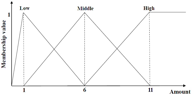
Fuzzy membership function
Why FFI-Miner is useful?
In real-life situations, it is difficult to handle quantitative databases using crisp sets. Fuzzy-set theory is useful to handle quantitative databases. Based on the fuzzy-set theory, the fuzzy frequent itemset mining algorithm FFI-Miner was proposed. It relies on a designed fuzzy-list structure to discover fuzzy itemsets. Compared to previous works, FFI-Miner has excellent performance for the discovery of fuzzy itemsets.
Input file format
The input file format of FFI-Miner is defined as follows. It is a text file. Each line represents a transaction. Each line is composed of three sections, as follows.
- First, the items contained in the transaction are listed. An item is represented by a positive integer. Each item is separated from the next item by a single space. It is assumed that all items within a same transaction (line) are sorted according to a total order (e.g. ascending order) and that no item can appear twice within the same transaction.
- Second, the symbol ":" appears and is followed by the sum of the quantities in that transaction.
- Third, the symbol ":" appears and is followed by the quantity of each item in this transaction (an integer), separated by single spaces.
For example, for the previous example, the input file is defined as follows:
1 3 4 5:26:5 10 2 9
1 2 3:13:8 2 3
2 3:12:3 9
1 2 3 5:21:5 3 10 3
1 3 4:19:7 9 3
2 3 4:13:2 8 3
1 2 3:12:5 2 5
1 3 4 5:19:3 10 2 2
Consider the first line. It means that the transaction {1, 3, 4, 5} has a total quantity of 26 and that items1, 3, 4 and 5 respectively have a quantity of 5, 10, 2 and 9 in this transaction. The following lines follow the same format.
Output file format
The output file format of FFI-Miner is defined as follows. It is a text file, where each line represents a fuzzy frequent itemset. On each line, the items of the itemset are first listed. Each item is represented by an integer, followed by “.” and either the letter “L”, “M” or “H”. These letters are used to indicate if an item is in the low-range, medium-range or high range in terms of the fuzzy membership function. After, all the items, the keyword "#FLV:" appears, which is followed by a float value indicating the fuzzy value of that itemset.
1.M #FVL: 4.2
1.M 2.L #FVL: 2.0
1.M 3.H #FVL: 2.6000001
2.L #FVL: 3.6
4.L #FVL: 2.8
4.L 3.H #FVL: 2.6000001
3.H #FVL: 4.0000005
For example, the first line indicates that the itemset 1 has a fuzzy value of 4.2 and is in the medium range of the fuzzy membership function. The other lines follow the same format.
Performance
FFI-Miner is a very efficient algorithm. It uses a designed fuzzy-list structure to identify unpromising candidates early, and thus speed up the discovery of fuzzy itemsets.
Where can I get more information about the algorithm?
This is the reference of the article describing the FFI-Miner algorithm:
Jerry Chun-Wei Lin, Ting Li, Philippe Fournier-Viger, and Tzung-Pei Hong. A Fast Algorithm for Mining Fuzzy Frequent Itemsets[J]. Journal of Intelligent & Fuzzy Systems, 2015, 29(6):2373-2379.
Example # 66: Mining Multiple Fuzzy Frequent Itemsets in a quantitative transaction database using the MFFI-Miner algorithm
How to run this example?
- If you are using the graphical interface, (1) choose the "MFFI-Miner" algorithm, (2) select the input file "contextMFFIMiner.txt", (3) set the output file name (e.g. "output.txt"), (4) set the minsup parameter to 2, and (5) click "Run algorithm".
- If you want to execute this example from the command line, then execute this command:
java -jar spmf.jar run MFFI-Miner contextMFFIMiner.txt output.txt 2 in a folder containing spmf.jar and the example input file contextMFFIMiner.txt .
- If you are using the source code version of SPMF, launch the file "MainTestMFFIMiner_saveToFile.java" in the package ca.pfv. SPMF.tests.
What is MFFI-Miner?
MFFI-Miner is an algorithm for mining fuzzy frequent itemsets in quantitative transactional database. In simple words, a quantitative transactional database is a database where items have quantities.
What is the input?
MFFI-Miner takes as input (1) a transaction database with quantity information and a minimum support threshold minSupport (a positive integer). Let's consider the following database consisting of 8 transactions (t1, t2, ..., t8) and 5 items (1, 2, 3, 4, 5). This database is provided in the text file “contextMFFIMiner.txt ” in the package ca.pfv.spmf.tests of the SPMF distribution.
Moreover, consider the membership function, shown below, which defines three ranges (low, medium, high).
Transaction ID |
Items |
Quantitates |
t1 |
3 4 5 |
3 2 1 |
t2 |
2 3 4 |
1 2 1 |
t3 |
2 3 5 |
3 3 1 |
t4 |
1 3 4 |
3 5 3 |
t5 |
1 2 3 4 |
1 1 2 1 |
t6 |
2 4 5 |
1 1 2 |
t7 |
1 2 4 5 |
4 3 5 3 |
t8 |
2 3 4 |
1 2 1 |
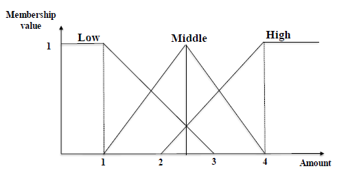
Fuzzy membership function
Why MFFI-Miner is useful?
Previous work on fuzzy frequent itemset mining used the maximum scalar cardinality to mine fuzzy frequent itemsets (FFIs), in which at most, only one linguistic term was used to represent the item in the databases. Although this process can reduce the amount of computation for mining FFIs, the discovered information may be invalid or incomplete. A gradual data-reduction approach (GDF) for mining multiple fuzzy frequent itemsets (MFFIs).The tree-based algorithm UBMFFP-tree suffered from building a huge tree structure. It mines FFIs with multiple fuzzy regions based on an Apriori-like mechanism. The MFFI-Miner algorithm efficiently mines MFFIs without candidate generation based on the designed fuzzy-list structure. This approach can be used to reduce the amount of computation and avoid using a generate-candidate-and-test approach with a level-wise exploration of the search space
Input file format
The input file format of MFFI-Miner is defined as follows. It is a text file. Each lines represents a transaction. Each line is composed of three sections, as follows.
- First, the items contained in the transaction are listed. An item is represented by a positive integer. Each item is separated from the next item by a single space. It is assumed that all items within a same transaction (line) are sorted according to a total order (e.g. ascending order) and that no item can appear twice within the same transaction.
- Second, the symbol ":" appears and is followed by the sum of the item quantities (an integer).
- Third, the symbol ":" appears and is followed by the quantity of each item in this transaction (an integer), separated by single spaces.
For example, for the previous example, the input file is defined as follows:
3 4 5:6:3 2 1
2 3 4:4:1 2 1
2 3 5:7:3 3 1
1 3 4:11:3 5 3
1 2 3 4:5:1 1 2 1
2 4 5:4:1 1 2
1 2 4 5:15:4 3 5 3
2 3 4:4:1 2 1
Consider the first line. It means that the transaction {3, 4, 5} has a total quantity of 6 and that items 3, 4 and 5 respectively have a quantity of 3, 2 and 1 in this transaction. The following lines follow the same format.
Output file format
The output file format of MFFI-Miner is defined as follows. It is a text file, where each line represents a frequent itemset. On each line, the items of the itemset are first listed. Each item is represented by an integer, followed by the letter "L", "M" or "H", and a single space. The letters L, M and H indicate if an item is in the Low, Medium or High Range of the fuzzy membership function, respectively. After, all the items, the keyword "#SUP:" appears, which is followed by a integer value indicating the support of that itemset.
3.H #SUP: 2.0
2.L #SUP: 4.0
2.L 3.M #SUP: 2.0
2.L 3.M 4.L #SUP: 2.0
2.L 4.L #SUP: 4.0
3.M #SUP: 3.3333335
3.M 4.L #SUP: 2.5000002
5.L #SUP: 2.5
4.L #SUP: 4.5
For example, the first line indicates that the itemset 3 in the high range of the fuzzy membership function (H) has a fuzzy value of 2.0. The other lines follows the same format.
Performance
MFFI-Miner is a very efficient algorithm. It uses a designed fuzzy-list structure to identify unpromising candidates early, and thus speed up the discovery of fuzzy itemsets.
Where can I get more information about the algorithm?
This is the article describing the MFFI-Miner algorithm:
Jerry Chun-Wei Lin, Ting Li, Philippe Fournier-Viger, Tzung-Pei Hong, Jimmy Ming-Thai Wu, and Justin Zhan. Efficient Mining of Multiple Fuzzy Frequent Itemsets[J]. International Journal of Fuzzy Systems, 2016:1-9.
Some other related papers:
T. P. Hong, G. C. Lan, Y. H. Lin, and S. T. Pan, An effective gradual data-reduction strategy for fuzzy itemset mining, International Journal of Fuzzy Systems, Vol. 15(2), pp.170-181, 2013. (GDF)
J. C. W. Lin, T. P. Hong, T. C. Lin, and S. T. Pan, An UBMFFP tree for mining multiple fuzzy frequent itemsets, International Journal of Uncertainty, Fuzziness and Knowledge- Based Systems, Vol. 23(6), pp. 861-879, 2015. (UBMFFP-tree)
Example 67 : Mining All Association Rules with the Lift
Measure
How to run this example?
- If you are using the graphical interface, (1)
choose the "FPGrowth_association_rules_with_lift"
algorithm , (2) select the input file "contextIGB.txt",
(3) set the output file name (e.g. "output.txt")
(4) set minsup = 50 %, minconf= 90% and minlift = 1 (5) click
"Run algorithm".
- If you want to execute this example from the command line,
then execute this command:
java -jar spmf.jar run FPGrowth_association_rules_with_lift
contextIGB.txt output.txt 50% 90% 1 in a folder
containing spmf.jar and the example input
file contextIGB.txt.
- If you are using the source code version of SPMF, launch
the file "MainTestAllAssociationRules_FPGrowth_version_with_lift.java"
in the package ca.pfv.SPMF.tests.
What is this algorithm?
This is a variation of the algorithm for mining all association
rules from a transaction database, described in the previous example.
Traditionally, association rule mining is performed by using two
interestingness measures named the support and confidence
to evaluate rules. In this example, we show how to use
another popular measure that is called the lift or interest.
What is the input?
The input is a transaction database (aka binary context) and three
thresholds named minsup (a value between 0 and 1),
minconf (a value between 0 and 1) and minlift (a value
between -infinity to +infinity).
A transaction database is a set of transactions.
Each transaction is a set of distinct items. For
example, consider the following transaction database. It contains 6
transactions (t1, t2, ..., t5, t6) and 5 items (1,2, 3, 4, 5). For
example, the first transaction represents the set of items 1, 2, 4 and
5. This database is provided as the file contextIGB.txt
in the SPMF distribution. It is important to note that an item is not
allowed to appear twice in the same transaction and that items are
assumed to be sorted by lexicographical order in a transaction.
| Transaction id |
Items |
| t1 |
{1, 2, 4, 5} |
| t2 |
{2, 3, 5} |
| t3 |
{1, 2, 4, 5} |
| t4 |
{1, 2, 3, 5} |
| t5 |
{1, 2, 3, 4, 5} |
| t6 |
{2, 3, 4} |
What is the output ?
The output of this algorithm is a set of all the association rules
that have a support, confidence and lift respectively higher than minsup,
minconf and minlift.
The lift of a rule X-->Y is calculated as
lift(X-->Y) = ( (sup(X U Y)/ N) / (sup(X)/ N*sup(Y)/ N ), where
- N is the number of transactions in the transaction database,
- sup(X∪Y) is the number of transactions containing X and Y,
- sup(X) is the number of transactions containing X
- sup(Y) is the number of transactions containing Y.
The confidence of a rule X-->Y is calculated
as conf(X-->Y) = sup(X U Y) / (sup(X)).
The support of a rule X -->Y is defined as
sup(X-->Y) = sup(X∪Y) / N
By applying the algorithm with minsup = 0.5, minconf=
0.9 and minlift = 1 on the previous database, we obtains 18
associations rules:
  rule 0:   4  ==> 2      support :  0.66 (4/6) confidence :  1.0  lift :  1.0
  rule 1:   3  ==> 2      support :  0.66 (4/6) confidence :  1.0  lift :  1.0
  rule 2:   1  ==> 5      support :  0.66 (4/6) confidence :  1.0  lift :  1.2
  rule 3:   1  ==> 2      support :  0.66 (4/6) confidence :  1.0  lift :  1.0
  rule 4:   5  ==> 2      support :  0.833(5/6)  confidence :  1.0  lift :  1.0
  rule 5:   4 5  ==> 2    support :  0.5 (3/6)   confidence :  1.0  lift :  1.0
  rule 6:   1 4  ==> 5    support :  0.5 (3/6)   confidence :  1.0  lift :  1.2
  rule 7:   4 5  ==> 1    support :  0.5 (3/6)   confidence :  1.0  lift :  1.5
  rule 8:   1 4  ==> 2    support :  0.5 (3/6)   confidence :  1.0  lift :  1.0
  rule 9:   3 5  ==> 2    support :  0.5 (3/6)   confidence :  1.0  lift :  1.0
  rule 10:  1 5  ==> 2    support :  0.66 (4/6)  confidence :  1.0  lift :  1.0
  rule 11:  1 2  ==> 5    support :  0.66 (4/6)  confidence :  1.0  lift :  1.2
  rule 12:  1  ==> 2 5    support :  0.66 (4/6)  confidence :  1.0  lift :  1.2
  rule 13:  1 4 5  ==> 2  support :  0.5 (3/6)   confidence :  1.0  lift :  1.0
  rule 14:  1 2 4  ==> 5  support :  0.5 (3/6)   confidence :  1.0  lift :  1.2
  rule 15:  2 4 5  ==> 1  support :  0.5 (3/6)   confidence :  1.0  lift :  1.5
  rule 16:  4 5  ==> 1 2  support :  0.5 (3/6)   confidence :  1.0  lift :  1.5
  rule 17:  1 4  ==> 2 5  support :  0.5 (3/6)   confidence :  1.0  lift :  1.5
How to interpret the results?
For an association rule X ==> Y, if the lift is equal
to 1, it means that X and Y are independent. If the lift is higher than
1, it means that X and Y are positively correlated. If the lift is
lower than 1, it means that X and Y are negatively correlated. For
example, if we consider the rule {1, 4} ==> {2, 5}, it has a lift of
1.5, which means that the occurrence of the itemset {1, 4} is
positively correlated with the occurrence of {2, 5}.
Input file format
The input file format is a text file containing
transactions. Each lines represents a transaction. The items in the
transaction are listed on the corresponding line. An item is
represented by a positive integer. Each item is separated from the
following item by a space. It is assumed that items are sorted
according to a total order and that no item can appear twice in the
same transaction. For example, for the previous example, the input file
is defined as follows:
1 2 4 5
2 3 5
1 2 4 5
1 2 3 5
1 2 3 4 5
2 3 4
Consider the first line. It means that the first transaction is
the itemset {1, 2, 4 and 5}. The following lines follow the same format.
Note that it is also possible to use the ARFF format
as an alternative to the default input format. The specification of the
ARFF format can be found here.
Most features of the ARFF format are supported except that (1) the
character "=" is forbidden and (2) escape characters are not
considered. Note that when the ARFF format is used, the performance of
the data mining algorithms will be slightly less than if the native
SPMF file format is used because a conversion of the input file will be
automatically performed before launching the algorithm and the result
will also have to be converted. This cost however should be small.
Output file format
The output file format is defined as follows. It
is a text file, where each line represents an association rule.
On each line, the items of the rule antecedent are first listed. Each
item is represented by an integer, followed by a single space. After,
that the keyword "==>" appears followed by a space. Then, the items
of the rule consequent are listed. Each item is represented by an
integer, followed by a single space. Then, the keyword " #SUP: "
appears followed by the support of the rule represented by an integer.
Then, the keyword " #CONF: " appears followed by the confidence of the
rule represented by a double value (a value between 0 and 1,
inclusively). Then, the keyword " #LIFT: " appears followed by the lift
of the rule represented by a double value (a value between -infinity to
+infinity). For example, here is a few lines from the output file for
this example:
1 ==> 2 4 5 #SUP: 3 #CONF: 0,75 #LIFT: 1,5
5 ==> 1 2 4 #SUP: 3 #CONF: 0,6 #LIFT: 1,2
For example, the first line indicates that the association rule
{1} --> {2, 4, 5} has a support of 3 transactions, a confidence of
75 % and a lift of 1.5 indicating a positive correlation (when the
value is higher than 1). The other lines follow the same format.
Note that if the ARFF format is used as input instead of the
default input format, the output format will be the same except that
items will be represented by strings instead of integers.
Implementation details
In the source code version of SPMF, there are two versions of this
algorithm. The first version saves the result into memory ("MainTestAllAssociationRules_FPGrowth_wifthLift").
The second one saves the result to a file ("MainTestAllAssociationRules_FPGrowth_saveToFile_wifthLift").
Note that we offer also the alternative of choosing CFPGrowth++
instead of FPGrowth. This is called the "CFPGrowth++_association_rules_lift"
algorithm in the graphical user interface or command line
interface. CFPGrowth++ allows to use multiple minimum
support thresholds instead of a single minsup threshold so the input
and output are slightly different (see the example about CFPGrowth++
for more details about this algorithm).
Where can I get more information about this algorithm?
The following technical report published in 1994 describes how to
generate association rules from frequent itemsets (Step 2):
R. Agrawal and R. Srikant. Fast algorithms for mining association rules in large
databases. Research Report RJ 9839, IBM Almaden Research Center,
San Jose, California, June 1994.
You can also read chapter 6
of the book "introduction to data mining" which provide a nice and
easy to understand introduction to how to discover frequent itemsets
and generate association rules, and also describes the advantages of
using the lift measure.
The following article describes the FPGrowth algorithm for mining
frequent itemsets:
Jiawei Han, Jian Pei, Yiwen Yin, Runying Mao: Mining
Frequent Patterns without Candidate Generation: A Frequent-Pattern Tree
Approach. Data Min. Knowl. Discov. 8(1): 53-87 (2004)
Example 68 :
Mining All Association Rules using the GCD algorithm
How to run this example?
- If you are using the graphical interface, (1)
choose the "GCD_association_rules" algorithm, (2) select the input file "contextIGB.txt",
(3) set the output file name (e.g. "output.txt")
(4) set minsup = 50 %, minconf= 60%, maxcomb = 3, and (5) click "Run
algorithm".
- If you want to execute this example from the command line,
then execute this command:
java -jar spmf.jar run GCD_association_rules contextIGB.txt output.txt 50% 60% 3 in a folder
containing spmf.jar and the example input
file contextIGB.txt.
- If you are using the source code version of SPMF, launch
this file "MainTestGCDAssociationRules.java" in the package ca.pfv.SPMF.tests.
What is this algorithm?
This algorithm finds the association rules in a given transaction database or sequence of transactions/events, using GCD calculations for prime numbers.It is an original algorithm implemented by Ahmed El-Serafy and Hazem El-Raffiee.
What is the input?
The input is a transaction database (aka binary context) and three
thresholds named minsup (a value between 0 and 1), minconf (a value between 0 and 1), and maxcomb (a positive integer).
A transaction database is a set of transactions.
Each transaction is a set of distinct items. For
example, consider the following transaction database. It contains 6
transactions (t1, t2, ..., t5, t6) and 5 items (1,2, 3, 4, 5). For
example, the first transaction represents the set of items 1, 2, 4 and
5. This database is provided as the file contextIGB.txt in the SPMF distribution. It is important to note that an item is not
allowed to appear twice in the same transaction and that items are
assumed to be sorted by lexicographical order in a transaction.
| Transaction id |
Items |
| t1 |
{1, 2, 4, 5} |
| t2 |
{2, 3, 5} |
| t3 |
{1, 2, 4, 5} |
| t4 |
{1, 2, 3, 5} |
| t5 |
{1, 2, 3, 4, 5} |
| t6 |
{2, 3, 4} |
What is the output?
The output of an association rule mining algorithm is a set of
association rules respecting the user-specified minsup and minconf thresholds. To explain how this algorithm works, it is necessary to
review some definitions. An association rule X==>Y
is a relationship between two itemsets (sets of items) X and Y such
that the intersection of X and Y is empty. The support of a
rule is the number of transactions that contains X∪Y. The confidence
of a rule is the number of transactions that contains X∪Y
divided by the number of transactions that contain X.
If we apply an association rule mining algorithm, it will return
all the rules having a support and confidence respectively no less than minsup and minconf.
For example, by applying the algorithm with minsup = 0.5 (50%),
minconf = 0.6 (60%), and maxcomb = 3, we obtain 56 associations rules (run
the example in the SPMF distribution to see the result).
Now let's explain the "maxcomb" parameter taken by the GCD algorithm. This parameter is used by the algorithm when finding the GCD (greatest common divisors) between two transactions. For example, consider 385, which comes from the multiplication of (5, 7 and 11), this actually means that (5), (7), (11), (5, 7), (5, 11), (7, 11), (5, 7, 11) are all common combinations between these two transactions. For larger GCD's, calculating all combinations grows exponentially in both time and memory. Hence, we introduced this parameter, to limit the maximum combinations' length generated from a single GCD. Although increasing this number might seem to provide more accurate results, the experiments showed that larger association rules occur at lower support (less important to the user). Hence, setting this parameter to values from 1 to 4 produces reasonable results.
Input file format
The input file format is a text file containing
transactions. Each lines represents a transaction. The items in the
transaction are listed on the corresponding line. An item is
represented by a positive integer. Each item is separated from the
following item by a space. It is assumed that items are sorted
according to a total order and that no item can appear twice in the
same transaction. For example, for the previous example, the input file
is defined as follows:
1 2 4 5
2 3 5
1 2 4 5
1 2 3 5
1 2 3 4 5
2 3 4
Consider the first line. It means that the first transaction is
the itemset {1, 2, 4 and 5}. The following lines follow the same format.
Note that it is also possible to use the ARFF format as an alternative to the default input format. The specification of the
ARFF format can be found here.
Most features of the ARFF format are supported except that (1) the
character "=" is forbidden and (2) escape characters are not
considered. Note that when the ARFF format is used, the performance of
the data mining algorithms will be slightly less than if the native
SPMF file format is used because a conversion of the input file will be
automatically performed before launching the algorithm and the result
will also have to be converted. This cost however should be small.
Output file format
The output file format is defined as follows. It
is a text file, where each line represents an association rule.
On each line, the items of the rule antecedent are first listed. Each
item is represented by an integer, followed by a single space. After,
that the keyword "==>" appears followed by a space. Then, the items
of the rule consequent are listed. Each item is represented by an
integer, followed by a single space. Then, the keyword " #SUP: "
appears followed by the support of the rule represented by an integer.
Then, the keyword " #CONF: " appears followed by the confidence of the
rule represented by a double value (a value between 0 and 1,
inclusively). For example, here is a few lines from the output file for
this example:
1 ==> 2 4 5 #SUP: 3 #CONF: 0,75
5 ==> 1 2 4 #SUP: 3 #CONF: 0,6
4 ==> 1 2 5 #SUP: 3 #CONF: 0,75
For example, the first line indicates that the association rule
{1} --> {2, 4, 5} has a support of 3 transactions and a confidence
of 75 %. The other lines follow the same format.
Note that if the ARFF format is used as input instead of the
default input format, the output format will be the same except that
items will be represented by strings instead of integers.
Where can I get more information about this algorithm?
The GCD Association Rules algorithm is an original algorithm. More information about it can be obtained from the bitbucket repository dedicated to this algorithm: https://bitbucket.org/aelserafy/gcd-association-rules
Example 69 : Mining the IGB basis of Association Rules
How to run this example?
- If you are using the graphical interface, (1)
choose the "IGB"
algorithm , (2) select the input file "contextIGB.txt",
(3) set the output file name (e.g. "output.txt")
(4) set minsup = 50 %, minconf= 61% (5) click "Run algorithm".
- If you want to execute this example from the command line,
then execute this command:
java -jar spmf.jar run IGB contextIGB.txt
output.txt 50% 61% in a folder containing spmf.jar
and the example input file contextIGB.txt.
- To run this example with the source code version of SPMF,
launch the file "MainTestIGB_saveToMemory.java"
in the package ca.pfv.SPMF.tests.
What is this algorithm?
This algorithm mines a subset of all association rules that is
called IGB association rules (Informative and Generic Basis of
Association Rules) from a transaction database.
To discover the IGB association rules, this algorithm performs two
steps: (1) first it discovers Closed itemsets and their associated
generators by applying the Zart algorithm. Then (2), association rules
are generated by using closed itemsets and generators.
What is the input?
The input is a transaction database and two thresholds named minsup
(a value between 0 and 1) and minconf (a value between 0 and
1) .
A transaction database is a set of transactions.
Each transaction is a set of distinct items. For
example, consider the following transaction database. It contains 6
transactions (t1, t2, ..., t5, t6) and 5 items (1,2, 3, 4, 5). For
example, the first transaction represents the set of items 1, 2, 4 and
5. This database is provided as the file contextIGB.txt
of the SPMF distribution. It is important to note that an item is not
allowed to appear twice in the same transaction and that items are
assumed to be sorted by lexicographical order in a transaction.
| Transaction id |
Items |
| t1 |
{1, 2, 4, 5} |
| t2 |
{2, 3, 5} |
| t3 |
{1, 2, 4, 5} |
| t4 |
{1, 2, 3, 5} |
| t5 |
{1, 2, 3, 4, 5} |
| t6 |
{2, 3, 4} |
What is the output?
The output is the IGB basis of association rules.
It is a compact set of association rules that is both informative and
generic. To explain what is the IGB basis of association rules, it is
necessary to review some definitions. An itemset is a
group of items. The support of an itemset is the
number of times that it appears in the database divided by the total
number of transactions in the database. For example, the itemset {1 3}
has a support of 33 % because it appears in 2 out of 6 transactions
from the database.
An association rule X--> Y is an association
between two itemsets X and Y that are disjoint. The support of
an association rule is the number of transactions that
contains X and Y divided by the total number of transactions. The
confidence of an association rule is the number of
transactions that contains X and Y divided by the number of
transactions that contains X.
A closed itemset is an itemset that is strictly
included in no itemset having the same support. An itemset Y is the
closure of an itemset X if Y is a closed itemset, X is a subset of Y
and X and Y have the same support. A generator Y of a
closed itemset X is an itemset such that (1) it has the same support as
X and (2) it does not have a subset having the same support.
The IGB set of association rules is the set of association rules
of the form X ==> Y - X, where X is a minimal generator of Y, Y is a
closed itemset having a support higher or equal to minsup,
and the confidence of the rule is higher or equal to minconf.
For example, by applying the IGB algorithm on
the transaction database previously described with minsup = 0.50 and
minconf= 0.61, we obtain the following set of association rules:
| Rule |
Support |
Confidence |
| 1 ==> 2, 4, 5 |
0.50 |
0.75 |
| 4 ==> 1, 2, 5 |
0.50 |
0.75 |
| 3 ==> 2, 5 |
0.50 |
0.75 |
| {} ==> 2, 3 |
0.66 |
0.66 |
| {} ==> 1, 2, 5 |
0.66 |
0.66 |
| {} ==> 2, 4 |
0.66 |
0.66 |
| {} ==> 2, 5 |
0.83 |
0.83 |
| {} ==> 2 |
1 |
1 |
Input file format
The input file format is a text file containing
transactions. Each lines represents a transaction. The items in the
transaction are listed on the corresponding line. An item is
represented by a positive integer. Each item is separated from the
following item by a space. It is assumed that items are sorted
according to a total order and that no item can appear twice in the
same transaction. For example, for the previous example, the input file
is defined as follows:
1 2 4 5
2 3 5
1 2 4 5
1 2 3 5
1 2 3 4 5
2 3 4
Consider the first line. It means that the first transaction is
the itemset {1, 2, 4 and 5}. The following lines follow the same format.
Note that it is also possible to use the ARFF format
as an alternative to the default input format. The specification of the
ARFF format can be found here.
Most features of the ARFF format are supported except that (1) the
character "=" is forbidden and (2) escape characters are not
considered. Note that when the ARFF format is used, the performance of
the data mining algorithms will be slightly less than if the native
SPMF file format is used because a conversion of the input file will be
automatically performed before launching the algorithm and the result
will also have to be converted. This cost however should be small.
Output file format
The output file format is defined as follows. It
is a text file, where each line represents an association rule.
On each line, the items of the rule antecedent are first listed. Each
item is represented by an integer, followed by a single space. After,
that the keyword "==>" appears followed by a space. Then, the items
of the rule consequent are listed. Each item is represented by an
integer, followed by a single space. Then, the keyword " #SUP: "
appears followed by the support of the rule represented by an integer.
Then, the keyword " #CONF: " appears followed by the confidence of the
rule represented by a double value (a value between 0 and 1,
inclusively). For example, here is a few lines from the output file for
this example:
1 ==> 2 4 5 #SUP: 0,5 #CONF: 0,75
3 ==> 2 5 #SUP: 3 #CONF: 0.75
For example, the first line indicates that the association rule
{1} --> {2, 4, 5} has a support of 3 transactions and a confidence
of 75 %. The other lines follow the same format.
Note that if the ARFF format is used as input instead of the
default input format, the output format will be the same except that
items will be represented by strings instead of integers.
Where can I get more information about IGB association rules?
This article described IGB rules:
G. Gasmi, S. Ben Yahia, E. Mephu Nguifo, Y. Slimani: IGB: A New
Informative Generic Base of Association Rules. PAKDD 2005: 81-90
Example 70 : Mining Perfectly Sporadic Association Rules
How to run this example?
- If you are using the graphical interface, (1)
choose the "Sporadic_association_rules"
algorithm , (2) select the input file "contextInverse.txt",
(3) set the output file name (e.g. "output.txt")
(4) set minsup = 1 %, maxsup = 60%, minconf= 60% (5)
click "Run algorithm".
- If you want to execute this example from the command line,
then execute this command:
java -jar spmf.jar run Sporadic_association_rules contextInverse.txt
output.txt 1% 60% 60% in a folder
containing spmf.jar and the example input
file contextInverse.txt.
- To run this example with the source code version of SPMF,
launch the file "MainTestAllPerfectlySporadicRules.java"
in the package ca.pfv.SPMF.tests.
What is this algorithm?
This is an algorithm for mining perfectly sporadic
association rules. The algorithm first uses AprioriInverse
to generate perfectly rare itemsets. Then, it uses these itemsets to
generate the association rules.
What is the input?
The input of this algorithm is a transaction
database and three thresholds named minusp, maxsup and minconf.
A transaction database is a set of transactions. A transaction is a set
of distinct items (symbols), assumed to be sorted in lexical order. For
example, the following transactions database contains 5 transactions
(t1,t2...t5) and 5 items (1,2,3,4,5). This database is provided in the
file "contextInverse.txt" of the SPMF distribution:
| Transaction id |
Items |
| t1 |
{1, 2, 4, 5} |
| t2 |
{1, 3} |
| t3 |
{1, 2, 3, 5} |
| t4 |
{2, 3} |
| t5 |
{1, 2, 4, 5} |
What is the output?
The output is the set of perfectly sporadic association
rules respecting the minconf (a value in [0,1]), minsup
(a value in [0,1]) and maxsup (a value in [0,1]) parameters.
To explain what it a perfectly sporadic association rule,
we need to review some definitions. An itemset is an
unordered set of distinct items. The support of an itemset is
the number of transactions that contain the itemset divided by the
total number of transactions. For example, the itemset {1, 2} has a
support of 60% because it appears in 3 transactions out of 5 (it
appears in t1, t2 and t5). A frequent itemset is an itemset that has a
support no less than the maxsup parameter.
A perfectly rare itemset (aka sporadic itemset)
is an itemset that is not a frequent itemset and that all its subsets
are also not frequent itemsets. Moreover, it has to have a support
higher or equal to the minsup threshold.
An association rule X==>Y is a relationship
between two itemsets (sets of items) X and Y such that the intersection
of X and Y is empty. The support of a rule is the
number of transactions that contains X∪Y divided by the total number of
transactions. The confidence of a rule is the number
of transactions that contains X∪Y divided by the number of transactions
that contain X.
A perfectly sporadic association rule X==>Y
is an association rule such that the confidence is higher or equal to minconf
and the support of any non empty subset of X∪Y is lower than maxsup.
For example, let's apply the algorithm with minsup = 0.1 %, maxsup
of 60 % and minconf = 60 %.
The first step that the algorithm perform is to apply AprioriInverse
algorithm with minsup = 0.1 % and maxsup of 60 %.
The result is the following set of perfectly rare itemsets:
| Perfectly Rare Itemsets |
Support |
| {3} |
60 % |
| {4} |
40 % |
| {5} |
60 % |
| {4, 5} |
40 % |
| {3, 5} |
20 % |
Then, the second step is to generate all perfectly sporadic
association rules respecting minconf by using the perfectly
rare itemsets found in the first step. The result is :
| Rule |
Support |
Confidence |
| 5 ==> 4 |
40 % |
60 % |
| 4 ==> 5 |
40 % |
100 % |
How to interpret the result?
For example, consider the rule 5 ==> 4. It means that if item 5
appears in a transaction, it is likely to be associated with item 4
with a confidence of 60 % (because 5 and 4 appears together in 40% of
the transactions where 5 appears). Moreover, this rule has a support of
40 % because it appears in 40% of the transactions of this database.
Input file format
The input file format is a text file containing
transactions. Each lines represents a transaction. The items in the
transaction are listed on the corresponding line. An item is
represented by a positive integer. Each item is separated from the
following item by a space. It is assumed that items are sorted
according to a total order and that no item can appear twice in the
same transaction. For example, for the previous example, the input file
is defined as follows:
1 2 4 5
1 3
1 2 3 5
2 3
1 2 4 5
Consider the first line. It means that the first transaction is
the itemset {1, 2, 4 and 5}. The following lines follow the same format.
Note that it is also possible to use the ARFF format
as an alternative to the default input format. The specification of the
ARFF format can be found here.
Most features of the ARFF format are supported except that (1) the
character "=" is forbidden and (2) escape characters are not
considered. Note that when the ARFF format is used, the performance of
the data mining algorithms will be slightly less than if the native
SPMF file format is used because a conversion of the input file will be
automatically performed before launching the algorithm and the result
will also have to be converted. This cost however should be small.
Output file format
The output file format is defined as follows. It
is a text file, where each line represents an association rule.
On each line, the items of the rule antecedent are first listed. Each
item is represented by an integer, followed by a single space. After,
that the keyword "==>" appears followed by a space. Then, the items
of the rule consequent are listed. Each item is represented by an
integer, followed by a single space. Then, the keyword " #SUP: "
appears followed by the support of the rule represented by an integer.
Then, the keyword " #CONF: " appears followed by the confidence of the
rule represented by a double value (a value between 0 and 1,
inclusively). For example, here is the output file for this example:
5 ==> 4 #SUP: 2 #CONF: 0,6
4 ==> 5 #SUP: 2 #CONF: 1
For example, the first line indicates that the association rule
{5} --> {4} has a support of 2 transactions and a confidence of 60
%. The second line follow the same format.
Note that if the ARFF format is used as input instead of the
default input format, the output format will be the same except that
items will be represented by strings instead of integers.
Where can I get more information about this algorithm?
The AprioriInverse algorithm and how to generate
sporadic rules are described in this paper:
Yun Sing Koh, Nathan Rountree: Finding Sporadic Rules Using Apriori-Inverse. PAKDD
2005: 97-106
Example 71 : Mining Closed Association Rules
How to run this example?
- If you are using the graphical interface, (1)
choose the "Closed_association_rules"
algorithm , (2) select the input file "contextZart.txt",
(3) set the output file name (e.g. "output.txt")
(4) set minsup = 60 %, minconf= 60% (5) click "Run algorithm".
- If you want to execute this example from the command line,
then execute this command:
java -jar spmf.jar run Closed_association_rules(using_fpclose) contextZart.txt
output.txt 60% 60% in a folder
containing spmf.jar and the example input
file contextZart.txt.
- To run this example with the source code version of SPMF,
launch the file "MainTestClosedAssociationRulesWithFPClose_saveToMemory.java"
in the package ca.pfv.SPMF.tests.
What is this algorithm?
It is an algorithm for mining "closed association rules",
which are a concise subset of all association rules.
What is the input of this algorithm?
The input is a transaction database (aka binary
context) and two thresholds named minsup (a
value in [0,1] that represents a percentage) and minconf
(a value in [0,1] that represents a percentage).
A transaction database is a set of transactions.
Each transaction is a set of distinct items. For
example, consider the following transaction database. It contains 5
transactions (t1, t2, ..., t5) and 5 items (1,2, 3, 4, 5). For example,
the first transaction represents the set of items 1, 2, 4 and 5. This
database is provided as the file contextZart.txt in
the SPMF distribution. It is important to note that an item is not
allowed to appear twice in the same transaction and that items are
assumed to be sorted by lexicographical order in a transaction.
| Transaction id |
Items |
| t1 |
{1, 2, 4, 5} |
| t2 |
{1, 3} |
| t3 |
{1, 2, 3, 5} |
| t4 |
{2, 3, 5} |
| t5 |
{1, 2, 3, 5} |
What is the output of this algorithm?
Given the minimum support threshold (minsup) and
minimum confidence threshold (minconf) set by the
user, the algorithm returns the set of closed association rules that
respect these thresholds. To explain what is a closed association rule,
it is necessary to review some definitions.
An itemset is an unordered set of distinct
items. The support of an itemset is the number of
transactions that contain the itemset divided by the total number of
transactions. For example, the itemset {1, 2} has a support of 60%
because it appears in 3 transactions out of 5 (it appears in t1, t2 and
t5). A closed itemset is an itemset that is strictly
included in no itemset having the same support.
An association rule X==>Y is a relationship
between two itemsets (sets of items) X and Y such that the intersection
of X and Y is empty. The support of a rule X==>Y
is the number of transactions that contains X∪Y divided by the total
number of transactions. The confidence of a rule
X==>Y is the number of transactions that contains X∪Y divided by the
number of transactions that contain X. A closed association
rule is an association rule of the form X ==> Y such that
the union of X and Y is a closed itemset.
The algorithm returns all closed association rules such that their
support and confidence are respectively higher or equal to the minsup
and minconf thresholds set by the user.
For instance, by applying this algorithm with minsup = 60 %,
minconf= 60%, we obtains 16 closed associations rules:
1 ==> 3 #SUP: 3 #CONF: 0.75 // which means that this rule has a
support of 3 transactions and a confidence of 75 %
3 ==> 1 #SUP: 3 #CONF: 0.75 // which means that this rule has a
support of 3 transactions and a confidence of 75 %
2 ==> 5 #SUP: 4 #CONF: 1.0 // which means that this rule has a
support of 4 transactions and a confidence of 100 %
5 ==> 2 #SUP: 4 #CONF: 1.0 // ...
2 5 ==> 1 #SUP: 3 #CONF: 0.75
1 5 ==> 2 #SUP: 3 #CONF: 1.0
1 2 ==> 5 #SUP: 3 #CONF: 1.0
1 ==> 2 5 #SUP: 3 #CONF: 0.75
2 ==> 1 5 #SUP: 3 #CONF: 0.75
5 ==> 1 2 #SUP: 3 #CONF: 0.75
3 5 ==> 2 #SUP: 3 #CONF: 1.0
2 3 ==> 5 #SUP: 3 #CONF: 1.0
2 5 ==> 3 #SUP: 3 #CONF: 0.75
5 ==> 2 3 #SUP: 3 #CONF: 0.75
3 ==> 2 5 #SUP: 3 #CONF: 0.75
2 ==> 3 5 #SUP: 3 #CONF: 0.75
Input file format
The input file format is a text file containing
transactions. Each lines represents a transaction. The items in the
transaction are listed on the corresponding line. An item is
represented by a positive integer. Each item is separated from the
following item by a space. It is assumed that items are sorted
according to a total order and that no item can appear twice in the
same transaction. For example, for the previous example, the input file
is defined as follows:
1 2 4 5
1 3
1 2 3 5
2 3 5
1 2 3 5
This file contains five lines (five transactions). Consider the
first line. It means that the first transaction is the itemset {1, 2,
4, 5}. The following lines follow the same format.
Note that it is also possible to use the ARFF format
as an alternative to the default input format. The specification of the
ARFF format can be found here.
Most features of the ARFF format are supported except that (1) the
character "=" is forbidden and (2) escape characters are not
considered. Note that when the ARFF format is used, the performance of
the data mining algorithms will be slightly less than if the native
SPMF file format is used because a conversion of the input file will be
automatically performed before launching the algorithm and the result
will also have to be converted. This cost however should be small.
Output file format
The output file format is defined as follows. It
is a text file, where each line represents an association rule.
On each line, the items of the rule antecedent are first listed. Each
item is represented by an integer, followed by a single space. After,
that the keyword "==>" appears followed by a space. Then, the items
of the rule consequent are listed. Each item is represented by an
integer, followed by a single space. Then, the keyword " #SUP: "
appears followed by the support of the rule represented by an integer.
Then, the keyword " #CONF: " appears followed by the confidence of the
rule represented by a double value (a value between 0 and 1,
inclusively). For example, here is the output file for this example:
1 ==> 3 #SUP: 3 #CONF: 0.75
3 ==> 1 #SUP: 3 #CONF: 0.75
2 ==> 5 #SUP: 4 #CONF: 1.0
5 ==> 2 #SUP: 4 #CONF: 1.0
1 2 ==> 5 #SUP: 3 #CONF: 1.0
2 5 ==> 1 #SUP: 3 #CONF: 0.75
1 5 ==> 2 #SUP: 3 #CONF: 1.0
5 ==> 1 2 #SUP: 3 #CONF: 0.75
2 ==> 1 5 #SUP: 3 #CONF: 0.75
1 ==> 2 5 #SUP: 3 #CONF: 0.75
2 5 ==> 3 #SUP: 3 #CONF: 0.75
2 3 ==> 5 #SUP: 3 #CONF: 1.0
3 5 ==> 2 #SUP: 3 #CONF: 1.0
5 ==> 2 3 #SUP: 3 #CONF: 0.75
2 ==> 3 5 #SUP: 3 #CONF: 0.75
3 ==> 2 5 #SUP: 3 #CONF: 0.75
For example, the last line indicates that the association rule {3}
--> {2, 5} has a support of 3 transactions and a confidence of 75 %.
The other lines follow the same format.
Note that if the ARFF format is used as input instead of the
default input format, the output format will be the same except that
items will be represented by strings instead of integers.
Implementation details and performance
There are two versions of this algorithms implemented in SPMF. The first one uses CHARM for finding the frequent closed itemsets before generating the rules. The second one uses FPClose for finding the frequent closed itemsets before generating the rules. The version based on FPClose is generally faster than the version based on CHARM.
In the release version of SPMF, the algorithm "Closed_association_rules(using_fpclose)" denotes the version using FPClose, while "Closed_association_rules" denotes the version based on CHARM.
In the source code version of SPMF, the files "MainTestClosedAssociationRulesWithFPClose_saveToMemory" and "MainTestClosedAssociationRulesWithFPClose_saveToFile" denotes respectively the version using FPClose which saves the result to memory or to a file. Moreover, the files "MainTestClosedAssociationRules_saveToMemory" and "MainTestClosedAssociationRules_saveToFile" denotes respectively the version using CHARM which saves the result to memory or to a file.
Where can I get more information about closed association rules?
The following Ph.D. thesis proposed "closed association
rules".
Szathmary, L. (2006). Symbolic Data Mining Methods with the Coron
Platform. Szathmary, L. PhD thesis, University Henri Poincaré — Nancy
1, France.
Example 72 : Mining Minimal Non Redundant Association
Rules
How to run this example?
- If you are using the graphical interface, (1)
choose the "MNR"
algorithm , (2) select the input file "contextZart.txt",
(3) set the output file name (e.g. "output.txt")
(4) set minsup = 60 %, minconf= 60% (5) click "Run algorithm".
- If you want to execute this example from the command line,
then execute this command:
java -jar spmf.jar run MNR contextZart.txt
output.txt 60% 60% in a folder
containing spmf.jar and the example input
file contextZart.txt.
- To run this example with the source code version of SPMF,
launch the file "MainTestMNRRules_saveToMemory.java"
in the package ca.pfv.SPMF.tests.
What is this algorithm?
This algorithm discover the set of "minimal non redundant
association rules" (Kryszkiewicz,
1998), which is a lossless and compact set of association rules.
In this implementation we use the Zart algorithm for discovering
closed itemsets and their associated generators. Then, this information
is used to generate the "minimal non redundant association rules".
What is the input?
The input is a transaction database (aka binary
context), a threshold named minconf
(a value in [0,1] that represents a percentage) and a
threshold named minsup (a
value in [0,1] that represents a percentage).
A transaction database is a set of transactions.
Each transaction is a set of items. For example,
consider the following transaction database. It contains 5 transactions
(t1, t2, ..., t5) and 5 items (1,2, 3, 4, 5). For example, the first
transaction represents the set of items 1, 2, 4 and 5. This database is
provided as the file contextZart.txt in the SPMF
distribution. It is important to note that an item is not allowed to
appear twice in the same transaction and that items are assumed to be
sorted by lexicographical order in a transaction.
| Transaction id |
Items |
| t1 |
{1, 2, 4, 5} |
| t2 |
{1, 3} |
| t3 |
{1, 2, 3, 5} |
| t4 |
{2, 3, 5} |
| t5 |
{1, 2, 3, 5} |
What is the output?
This algorithm returns the set of minimal non redundant
association rules.
To explain what is the set of minimal non redundant association
rules, it is necessary to review some definitions. An itemset
is a set of distinct items. The support of an itemset is
the number of times that it appears in the database divided by the
total number of transactions in the database. For example, the itemset
{1 3} has a support of 33 % because it appears in 2 out of 6
transactions from the database.
An association rule X--> Y is an association
between two itemsets X and Y that are disjoint. The support of
an association rule is the number of transactions that
contains X and Y divided by the total number of transactions. The
confidence of an association rule is the number of
transactions that contains X and Y divided by the number of
transactions that contains X.
A closed itemset is an itemset that is strictly
included in no itemset having the same support. An itemset Y is the
closure of an itemset X if Y is a closed itemset, X is a subset of Y
and X and Y have the same support. A generator Y of a
closed itemset X is an itemset such that (1) it has the same support as
X and (2) it does not have a subset having the same support.
The set of minimal non redundant association rules
is defined as the set of association rules of the form P1 ==> P2 /
P1, where P1 is a generator of P2, P2 is a closed itemset, and the rule
has a support and confidence respectively no less than minsup and
minconf.
For example, by applying this algorithm with minsup = 60 %,
minconf= 60% on the previous database, we obtains 14 minimal
non redundant associations rules:
2 3 ==> 5 support:: 0.6 confidence: 1
3 5 ==> 2 support: 0.6 confidence: 1
1 ==> 3 support: 0.6 confidence: 0,75
1 ==> 2 5 support: 0.6 confidence: 0,75
1 2 ==> 5 support: 0.6 confidence: 1
1 5 ==> 2 support: 0.6 confidence: 1
3 ==> 1 support: 0.6 confidence: 0,75
3 ==> 2 5 support: 0.6 confidence: 0,75
2 ==> 3 5 support: 0.6 confidence: 0,75
2 ==> 1 5 support: 0.6 confidence: 0,75
2 ==> 5 support: 0.8 confidence: 1
5 ==> 2 3 support: 0.6 confidence: 0,75
5 ==> 1 2 support: 0.6 confidence: 0,75
5 ==> 2 support: 0.8 confidence: 1
Input file format
The input file format is a text file containing
transactions. Each lines represents a transaction. The items in the
transaction are listed on the corresponding line. An item is
represented by a positive integer. Each item is separated from the
following item by a space. It is assumed that items are sorted
according to a total order and that no item can appear twice in the
same transaction. For example, for the previous example, the input file
is defined as follows:
1 2 4 5
1 3
1 2 3 5
2 3 5
1 2 3 5
This file contains five lines (five transactions). Consider the
first line. It means that the first transaction is the itemset {1, 2,
4, 5}. The following lines follow the same format.
Note that it is also possible to use the ARFF format
as an alternative to the default input format. The specification of the
ARFF format can be found here.
Most features of the ARFF format are supported except that (1) the
character "=" is forbidden and (2) escape characters are not
considered. Note that when the ARFF format is used, the performance of
the data mining algorithms will be slightly less than if the native
SPMF file format is used because a conversion of the input file will be
automatically performed before launching the algorithm and the result
will also have to be converted. This cost however should be small.
Output file format
The output file format is defined as follows. It
is a text file, where each line represents an association rule.
On each line, the items of the rule antecedent are first listed. Each
item is represented by an integer, followed by a single space. After,
that the keyword "==>" appears followed by a space. Then, the items
of the rule consequent are listed. Each item is represented by an
integer, followed by a single space. Then, the keyword " #SUP: "
appears followed by the support of the rule represented by an double
value indicating a p. Then, the keyword " #CONF: " appears followed by
the confidence of the rule represented by a double value (a value
between 0 and 1, inclusively). For example, here is the output file for
this example:
2 ==> 5 #SUP: 0,8 #CONF: 1
2 ==> 3 5 #SUP: 0,6 #CONF: 0,75
2 ==> 1 5 #SUP: 0,6 #CONF: 0,75
5 ==> 2 #SUP: 0,8 #CONF: 1
5 ==> 2 3 #SUP: 0,6 #CONF: 0,75
5 ==> 1 2 #SUP: 0,6 #CONF: 0,75
3 ==> 2 5 #SUP: 0,6 #CONF: 0,75
3 ==> 1 #SUP: 0,6 #CONF: 0,75
2 3 ==> 5 #SUP: 0,6 #CONF: 1
3 5 ==> 2 #SUP: 0,6 #CONF: 1
1 2 ==> 5 #SUP: 0,6 #CONF: 1
1 5 ==> 2 #SUP: 0,6 #CONF: 1
1 ==> 3 #SUP: 0,6 #CONF: 0,75
1 ==> 2 5 #SUP: 0,6 #CONF: 0,75
For example, the last line indicates that the association rule {1}
--> {2, 5} has a support of 60 % and a confidence of 75%. The other
lines follow the same format.
Note that if the ARFF format is used as input instead of the
default input format, the output format will be the same except that
items will be represented by strings instead of integers.
Where can I get more information about closed association rules?
The following article provides detailed information about
Minimal Non Redundant Association Rules:
M. Kryszkiewicz (1998). Representative
Association Rules and Minimum Condition Maximum Consequence Association
Rules. Proc. of PKDD '98, Nantes, France, September 23-26.
Example 73 : Mining Indirect Association Rules with the
INDIRECT algorithm
How to run this example?
- If you are using the graphical interface, (1)
choose the "Indirect_association_rules"
algorithm, (2) select the input file "contextIndirect.txt",
(3) set the output file name (e.g. "output.txt")
(4) set minsup = 60 %, ts = 50 % and minconf= 10%
(5) click "Run algorithm".
- If you want to execute this example from the command line,
then execute this command:
java -jar spmf.jar run Indirect_association_rules contextIndirect.txt
output.txt 60% 50% 10% in a folder containing spmf.jar and the example input file contextIndirect.txt.
- If you are using the source code version of SPMF, launch
the file "MainTestIndirectRules_saveToFile.java"
in the package ca.pfv.SPMF.tests.
What is the INDIRECT algorithm?
Indirect (Tan et al., KDD 2000; Tan, Steinbach
& Kumar, 2006, p.469) is an algorithm for discovering indirect
associations between items in transactions databases.
Why this algorithm is important? Because traditional association
rule mining algorithms focus on direct associations between itemsets.
This algorithm can discover indirect associations, which can be useful
in domains such as biology. Indirect association rule mining has
various applications such as stock market analysis and competitive
product analysis (Tan et al., 2000).
What is the input?
The input of the indirect algorithm is
a transaction database and three parameters named minsup (a
value in [0,1] that represents a percentage), ts (a value in
[0,1] that represents a percentage) and minconf (a value in
[0,1] that represents a percentage).
A transaction database is a set of transactions.
Each transaction is a set of distinct items. For
example, consider the following transaction database. It contains 5
transactions (t1, t2, ..., t5) and 5 items (1,2, 3, 4, 5). For example,
the first transaction represents the set of items 1, 4 and 5. This
database is provided as the file contextIndirect.txt
in the SPMF distribution. It is important to note that an item is not
allowed to appear twice in the same transaction and that items are
assumed to be sorted by lexicographical order in a transaction.
| Transaction id |
Items |
| t1 |
{1, 4, 5} |
| t2 |
{2, 3, 4} |
| t3 |
{1, 2, 4, 5} |
| t4 |
{5} |
| t5 |
{1, 2, 4, 5} |
The three numeric parameters of the indirect algorithm
are:
- minsup : called the "mediator minimum support".
- ts : called the "itempair minimum support"
- minconf : representing the minimal confidence required
for indirect associations (note that in the original article it uses
the IS measure instead of the confidence).
What is the output?
The result is all indirect associations
respecting the parameters minsup, ts and
minconf. An indirect association has the form
{x,y} ==> M, where x and y are single items and M is an itemset
called the "mediator".
An indirect association has to respect the
following conditions:
- The number of transactions containing all items of {x}∪ M
divided by the total number of transaction must be higher or equal to minsup.
- The number of transactions containing all items of {y}∪ M
divided by the total number of transaction must be higher or equal to minsup.
- The number of transactions containing {x,y} divided by the
total number of transaction must be smaller than ts.
- The confidence of {x}with respect to M and {y}with respect M
must be higher or equal to minconf. The confidence of an
itemset X with respect to another itemset Y is defined as the number of
transactions that contains X and Y divided by the number of
transactions that contain X.
For example, by applying the indirect algorithm with
minsup = 60 %, ts = 50 % and minconf= 10%, we
obtain 3 indirect association rules:
- {1, 2 | {4}}, which means that 1 and 2 are indirectly
associated by the mediator {4 }.
- {1, 5 | {4}}, which means that 1 and 5 are indirectly
associated by the mediator {4 }.
- {2, 5 | {4}}, which means that 1 and 5 are indirectly
associated by the mediator {4 }.
To see additional details about each of these three indirect
rules, run this example.
Input file format
The input file format is a text file containing
transactions. Each lines represents a transaction. The items in the
transaction are listed on the corresponding line. An item is
represented by a positive integer. Each item is separated from the
following item by a space. It is assumed that items are sorted
according to a total order and that no item can appear twice in the
same transaction. For example, for the previous example, the input file
is defined as follows:
1 4
2 3 4
1 2 4 5
4 5
1 2 4 5
This file contains five lines (five transactions). Consider the
first line. It means that the first transaction is the itemset {1, 4}.
The following lines follow the same format.
Note that it is also possible to use the ARFF format
as an alternative to the default input format. The specification of the
ARFF format can be found here.
Most features of the ARFF format are supported except that (1) the
character "=" is forbidden and (2) escape characters are not
considered. Note that when the ARFF format is used, the performance of
the data mining algorithms will be slightly less than if the native
SPMF file format is used because a conversion of the input file will be
automatically performed before launching the algorithm and the result
will also have to be converted. This cost however should be small.
Output file format
The output file format is defined as follows. It
is a text file, where each line represents an indirect
association rule. Each line starts by "(a=x b=y | mediator=M
)" indicating that the line represents the rule {x,y} ==> M,
where x, y and M are integers
representing items. Then, the keyword "#sup(a,mediator)=" is followed
by the support of {x}∪ M expressed as a number of
transactions (an integer). Then, the keyword "#sup(b,mediator)=" is
followed by the support of {y}∪ M expressed as a
number of transactions (an integer). Then, the keyword
"#conf(a,mediator)= " is followed by the confidence of a
with respect to the mediator, expressed as a double value in the [0, 1]
interval. Then, the keyword "#conf(b,mediator)= " appears followed by
the confidence of b with respect to the mediator,
expressed as a double value in the [0, 1] interval.
For example, the output file of this example is:
(a=1 b=2 | mediator=4 ) #sup(a,mediator)= 3 #sup(b,mediator)= 3
#conf(a,mediator)= 1.0 #conf(b,mediator)= 1.0
(a=1 b=5 | mediator=4 ) #sup(a,mediator)= 3 #sup(b,mediator)= 3
#conf(a,mediator)= 1.0 #conf(b,mediator)= 1.0
(a=2 b=5 | mediator=4 ) #sup(a,mediator)= 3 #sup(b,mediator)= 3
#conf(a,mediator)= 1.0 #conf(b,mediator)= 1.0
This file contains three lines (three indirect association rules).
Consider the first line. It represents that items 1 and 2 are
indirectly associated by the item 4 as mediator. Furthermore, it
indicates that the support of {1, 4} is 3 transactions, the support of
{2,4} is 3 transactions, the confidence of item 1 with respect to item
4 is 100 % and the confidence of item 2 with respect to item 4 is 100%.
The other lines follow the same format.
Note that if the ARFF format is used as input instead of the default
input format, the output format will be the same except that items will
be represented by strings instead of integers.
Implementation details
The implementation attempts to be as faithful as possible to the
original algorithm, except that the confidence is used instead of the
IS measure.
Note that some algorithms claimed to be more efficient than
Indirect such as HI-Mine but they have not been implemented in SPMF.
Where can I get more information about indirect association rules?
The concept of indirect associations was proposed by Tan (2000) in
this conference paper:
Pang-Ning Tan, Vipin Kumar, Jaideep Srivastava: Indirect
Association: Mining Higher Order Dependencies in Data. PKDD 2000:
632-637
Moreover, note that the book "Introduction do data mining" by Tan,
Steinbach and Kumar provides an overview of indirect association rules
that is easy to read.
Example 74 : Hiding Sensitive Association Rules with the
FHSAR algorithm
How to run this example?
- If you are using the graphical interface, (1)
choose the "FHSAR"
algorithm, (2) select the input file "contextIGB.txt",
(3) set the output file name (e.g. "output.txt")
(4) set minsup = 50 %, minconf= 60% and sar_file
= "sar.txt"(5) click "Run algorithm".
- If you want to execute this example from the command line,
then execute this command:
java -jar spmf.jar run FHSAR contextIGB.txt
output.txt 50% 60% sar.txt in a folder containing spmf.jar and the example input file contextIGB.txt.
- To run this example with the source code version of SPMF,
launch the file "MainTestFHSAR_saveToFile.java"
in the package ca.pfv.SPMF.tests.
What is FHSAR?
FHSAR is an algorithm for hiding sensitive association rules in a
transaction database.
What are the applications? For example, consider a company that
want to release a transaction database to the public. But it does not
want to disclose some sensitive associations between items that appear
in the database and that could give a competitive advantage to their
competitor. The FHSAR algorithm can hide these associations by
modifying the database.
What is the input?
The FHSAR algorithm is designed to hide sensitive association
rules in a transaction database so that they will not be found for a
given minsup and minconf threshold generally used
by association rule mining algorithms. The input are: minsup (a
value in [0,1] that represents a percentage), minconf (a
value in [0,1] that represents a percentage), a transaction
database and some sensitive association rules to be hidden.
A transaction database is a set of transactions.
Each transaction is a set of distinct items. For
example, consider the following transaction database. It contains 6
transactions (t1, t2, ..., t5, t6) and 5 items (1, 2, 3, 4, 5). For
example, the first transaction represents the set of items 1, 2, 4 and
5. This database is provided as the file contextIGB.txt
in the SPMF distribution. It is important to note that an item is not
allowed to appear twice in the same transaction and that items are
assumed to be sorted by lexicographical order in a transaction.
| Transaction id |
Items |
| t1 |
{1, 2, 4, 5} |
| t2 |
{2, 3, 5} |
| t3 |
{1, 2, 4, 5} |
| t4 |
{1, 2, 3, 5} |
| t5 |
{1, 2, 3, 4, 5} |
| t6 |
{2, 3, 4} |
An association rule X==>Yis an association
between two sets of items X and Y such that X and Y are disjoint. The support
of an association rule X==>Yis the number of transactions
that contains both X and Y divided by the total number of transactions.
The confidence of an association rule X==>Y is the
number of transactions that contains both X and Y divided by the number
of transactions that contain X. For example, the rule {1 2} ==> {4
5} has a support of 50 % because it appears in 3 transactions out of 5.
Furthermore, it has a confidence of 75 % because {1 2} appears in 4
transactions and {1, 2, 4, 5} appears in 3 transactions.
What is the output?
The output is a new transaction database such that the sensitive
rules will not be found if an association rule mining algorithm is
applied with minsup and minconf.
For example, we can apply FHSAR with the parameters minsup = 0.5
and minconf = 0.60 to hide the following association rules provided in
the file "sar.txt":
- 4 ==> 1
- 1 2 ==> 4 5
- 5 ==> 2
the result is a new transaction database where these rules are
hidden for the given thresholds minsup and minconf:
| Transaction id |
Items |
| t1 |
{4, 5} |
| t2 |
{3, 5} |
| t3 |
{4, 5} |
| t4 |
{1, 2, 3, 5} |
| t5 |
{1, 2, 3, 4, 5} |
| t6 |
{2, 3, 4} |
Note that the result of the algorithm is not always the same
because I use the HashSet data structure to represent transactions
internally and this data structure do not keep the order. Therefore,
the items that are removed may not be the same if the algorithm is run
twice.
Input file format
This algorithm takes two files as input.
The first file is a text file containing
transactions (a transaction database) (e.g. contextIGB.txt).
Each line represents a transaction. The items in the transaction are
listed on the corresponding line. An item is represented by a positive
integer. Each item is separated from the following item by a space. It
is assumed that items are sorted according to a total order and that no
item can appear twice in the same transaction. For example, for the
previous example, the input file is defined as follows:
1 2 4 5
2 3 5
1 2 4 5
1 2 3 5
1 2 3 4 5
2 3 4
This file contains six lines (six transactions). Consider the
first line. It means that the first transaction is the itemset {1, 2,
4, 5}. The following lines follow the same format.
The second file is a text file containing
sensitive association rules to be hidden (e.g. sar.txt).
Each line is an association rule. First, the rule antecedent is
written. It is an itemset, where each item is represented by a positive
integer, and each item is separated from the following item by a single
space. Note that it is assumed that items within an itemset cannot
appear more than once and are sorted according to a total order. Then
the keyword " ==> " appears followed by the rule consequent. The
consequent is an itemset where each item is represented by a positive
integer, and each item is separated from the following item by a single
space. For example, consider the file sar.txt.
4 ==> 1
1 2 ==> 4 5
5 ==> 2
This file contains three lines (three association rules). The
second line indicates that the rule {1, 2} ==> {4, 5} should be
hidden by the FHSAR algorithm.
Output file format
The output file format is defined as follows. It
is a text file representing a transaction database. Each line
represents a transaction. The items in the transaction are listed on
the corresponding line. An item is represented by a positive integer.
Each item is separated from the following item by a space. It is
assumed that items are sorted according to a total order and that no
item can appear twice in the same transaction. For example, for the
previous example, an output file generated by the FHSAR algorithm is:
4 5
3 5
4 5
1 2 3 5
1 2 3 4 5
2 3 4
In this example, the first line represents the transaction {4, 5}.
Other lines follow the same format.
Where can I get more information about the FHSAR algorithm?
This algorithm was proposed in this paper:
C.-C.Weng, S.-T. Chen, H.-C. Lo: A Novel
Algorithm for Completely Hiding Sensitive Association Rules. ISDA
(3) 2008: 202-208
Example 75 : Mining the Top-K Association Rules
How to run this example?
- If you are using the graphical interface, (1)
choose the "TopKRules"
algorithm, (2) select the input file "contextIGB.txt",
(3) set the output file name (e.g. "output.txt")
(4) set k = 2 and minconf = 0.8 (5) click "Run algorithm".
- If you want to execute this example from the command line,
then execute this command:
java -jar spmf.jar run TopKRules contextIGB.txt
output.txt 2 80% in a folder containing spmf.jar
and the example input file contextIGB.txt.
- If you are using the source code version of SPMF, launch
the file "MainTestTopKRules.java"
in the package ca.pfv.SPMF.tests.
What is TopKRules?
TopKRules is an algorithm for discovering the top-k
association rules appearing in a transaction database.
Why is it useful to discover top-k association rules? Because
other association rule mining algorithms requires to set a minimum
support (minsup) parameter that is hard to set (usually users
set it by trial and error, which is time consuming). TopKRules
solves this problem by letting users directly indicate k, the
number of rules to be discovered instead of using minsup.
What is the input of TopKRules ?
TopKRules takes three parameters as input:
- a transaction database,
- a parameter k representing the number of association
rules to be discovered (a positive integer),
- a parameter minconf representing the minimum
confidence that the association rules should have (a value in [0,1]
representing a percentage).
A transaction database is a set of transactions.
Each transaction is a set of items. For example,
consider the following transaction database. It contains 6 transactions
(t1, t2, ..., t5, t6) and 5 items (1,2, 3, 4, 5). For example, the
first transaction represents the set of items 1, 2, 4 and 5. This
database is provided as the file contextIGB.txt in
the SPMF distribution. It is important to note that an item is not
allowed to appear twice in the same transaction and that items are
assumed to be sorted by lexicographical order in a transaction.
| Transaction id |
Items |
| t1 |
{1, 2, 4, 5} |
| t2 |
{2, 3, 5} |
| t3 |
{1, 2, 4, 5} |
| t4 |
{1, 2, 3, 5} |
| t5 |
{1, 2, 3, 4, 5} |
| t6 |
{2, 3, 4} |
What is the output of TopKRules ?
TopKRules outputs the top-k association
rules.
To explain what are top-k association rules, it
is necessary to review some definitions. An itemset
is a set of distinct items. The support of an itemset is
the number of times that it appears in the database divided by the
total number of transactions in the database. For example, the itemset
{1 3} has a support of 33 % because it appears in 2 out of 6
transactions from the database.
An association rule X--> Y is an association
between two itemsets X and Y that are disjoint. The support of
an association rule is the number of transactions that
contains X and Y divided by the total number of transactions. The
confidence of an association rule is the number of
transactions that contains X and Y divided by the number of
transactions that contains X.
The top-k association rules are the k most
frequent association rules in the database having a
confidence higher or equal to minconf.
For example, if we run TopKRules with k = 2
and minconf = 0.8, we obtain the top-2 rules in the
database having a confidence higher or equals to 80 %.
- 2 ==> 5, which have a support of 5 (it appears in 5
sequences) and a confidence of 83%
- 5 ==> 2, which have a support of 5 (it appears in 5
sequences) and a confidence of 100 %
For instance, the rule 2 ==>5 means that if item 2 appears, it
is likely to be associated with item 5 with a confidence of 83% in a
transaction. Moreover, this rule has a support of 83 % because it
appears in five transactions (S1, S2 and S3) out of the six
transactions contained in this database.
It is important to note that for some values of k, the
algorithm may return slightly more than k rules. This is can
happen if several rules have exactly the same support.
Input file format
The input file format is a text file containing
transactions. Each lines represents a transaction. The items in the
transaction are listed on the corresponding line. An item is
represented by a positive integer. Each item is separated from the
following item by a space. It is assumed that items are sorted
according to a total order and that no item can appear twice in the
same transaction. For example, for the previous example, the input file
is defined as follows:
1 2 4 5
2 3 5
1 2 4 5
1 2 3 5
1 2 3 4 5
2 3 4
Consider the first line. It means that the first transaction is
the itemset {1, 2, 4 and 5}. The following lines follow the same format.
Note that it is also possible to use the ARFF format
as an alternative to the default input format. The specification of the
ARFF format can be found here.
Most features of the ARFF format are supported except that (1) the
character "=" is forbidden and (2) escape characters are not
considered. Note that when the ARFF format is used, the performance of
the data mining algorithms will be slightly less than if the native
SPMF file format is used because a conversion of the input file will be
automatically performed before launching the algorithm and the result
will also have to be converted. This cost however should be small.
Output file format
The output file format is defined as follows. It
is a text file, where each line represents an association rule.
On each line, the items of the rule antecedent are first listed. Each
item is represented by a positive integer, followed by a single space.
After, that the keyword "==>" appears followed by a space. Then, the
items of the rule consequent are listed. Each item is represented by an
integer, followed by a single space. Then, the keyword " #SUP: "
appears followed by the support of the rule represented by an integer
(a number of transactions). Then, the keyword " #CONF: " appears
followed by the confidence of the rule represented by a double value (a
value between 0 and 1, inclusively). For example, here is a few lines
from the output file if we run TopKRules on contextIGB.txt with k=2 and
minconf=0.8 (80 %):
2 ==> 5 #SUP: 5 #CONF: 0.8333333333333334
5 ==> 2 #SUP: 5 #CONF: 1.0
For example, the first line indicates that the association rule
{2} --> {5} has a support of 5 transactions and a confidence of 83.3
%. The other lines follow the same format.
Note that if the ARFF format is used as input instead of the
default input format, the output format will be the same except that
items will be represented by strings instead of integers.
Performance
TopKRules is a very efficient algorithm for
mining the top-k association rules.
It provides the benefits that it is very intuitive to use. It
should be noted that the problem of top-k association rule
mining is more computationally expensive than the problem of
association rule mining. Using TopKRules is recommended for k values
of up to 5000, depending on the datasets.
Besides, note that there is a variation of TopKRules
named TNR that is available in SPMF. The improvement
in TNR is that it eliminates some association rules that are deemed
"redundant" (rules that are included in other rules having the same
support and confidence - see the TNR example for the formal
definition). Using TNR is more costly than using TopKRules but it
brings the benefit of eliminating a type of redundancy in results.
Where can I get more information about this algorithm?
The TopKRules algorithm was proposed in this paper:
Fournier-Viger, P., Wu, C.-W., Tseng, V. S. (2012). Mining
Top-K Association Rules. Proceedings of the 25th Canadian Conf. on
Artificial Intelligence (AI 2012), Springer, LNAI 7310, pp. 61-73.
Example 76 : Mining the Top-K Non-Redundant Association
Rules
How to run this example?
- If you are using the graphical interface, (1)
choose the "TNR" algorithm,
(2) select the input file "contextIGB.txt", (3) set the output file name
(e.g. "output.txt") (4)
set k = 30,minconf = 0.5, and delta = 2 (5) click "Run algorithm".
- If you want to execute this example from the command line,
then execute this command:
java -jar spmf.jar run TNR contextIGB.txt
output.txt 30 0.5 2 in a folder containing spmf.jar
and the example input file contextIGB.txt.
- If you are using the source code version of SPMF, launch
the file "MainTestTNR.java"
in the package ca.pfv.SPMF.tests.
What is TopKRules?
TNR is an algorithm for discovering the top-k
non-redundant association rules appearing in a transaction
database. It is an approximate algorithm in the sense that it always
generates non-redundant rules. But these rules may not always be the
top-k non-redundant association rules. TNR uses a parameter named delta,
which is a positive integer >=0 that can be used to improve the
chance that the result is exact (the higher the delta value, the more
chances that the result will be exact).
Why is it important to discover top-k non-redundant
association rules? Because other association rule mining
algorithms requires that the user set a minimum support (minsup)
parameter that is hard to set (usually users set it by trial and error,
which is time consuming). Moreover, the result of association rule
mining algorithms usually contains a high level of redundancy (for
example, thousands of rules can be found that are variation of other
rules having the same support and confidence). The TNR
algorithm provide a solution to both of these problems by letting users
directly indicate k, the number of rules to be discovered,
and by eliminating redundancy in results.
What is the input of TNR ?
TNR takes four parameters as input:
- a transaction database,
- a parameter k representing the number of rules to be
discovered (a positive integer >= 1),
- a parameter minconf representing the minimum
confidence that association rules should have (a value in [0,1]
representing a percentage).
- a parameter delta (a positive integer >=0) that is
used to increase the chances of having an exact result (because the TNR
algorithm is approximate).
A transaction database is a set of transactions.
Each transaction is a set of items. For example,
consider the following transaction database. It contains 6 transactions
(t1, t2, ..., t5, t6) and 5 items (1,2, 3, 4, 5). For example, the
first transaction represents the set of items 1, 2, 4 and 5. This
database is provided as the file contextIGB.txt in
the SPMF distribution. It is important to note that an item is not
allowed to appear twice in the same transaction and that items are
assumed to be sorted by lexicographical order in a transaction.
| Transaction id |
Items |
| t1 |
{1, 2, 4, 5} |
| t2 |
{2, 3, 5} |
| t3 |
{1, 2, 4, 5} |
| t4 |
{1, 2, 3, 5} |
| t5 |
{1, 2, 3, 4, 5} |
| t6 |
{2, 3, 4} |
What is the output of TNS ?
TNR outputs an approximation of the k most
frequent non redundant association rules having a
confidence higher or equal to minconf.
To explain what are top-k non redundant association rules,
it is necessary to review some definitions. An itemset
is a set of distinct items. The support of an itemset is
the number of times that it appears in the database divided by the
total number of transactions in the database. For example, the itemset
{1 3} has a support of 33 % because it appears in 2 out of 6
transactions from the database.
An association rule X--> Y is an association
between two itemsets X and Y that are disjoint. The support of
an association rule is the number of transactions that
contains X and Y divided by the total number of transactions. The
confidence of an association rule is the number of
transactions that contains X and Y divided by the number of
transactions that contains X.
An association rule ra: X → Y is
redundant with respect to another rule rb : X1 → Y1
if and only if:
- conf(ra) = conf(rb)
- sup(ra) = sup(rb)
- X1 ⊆ X ∧ Y ⊆ Y1.
The top-k non redundant association rules are the
k most non-redundant frequent association rules
in the database having a confidence higher or equal to minconf.
For example, If we run TNR with k = 10
and minconf = 0.5 and delta = 2, the following set
of rules is found
4, ==> 2,  sup= 4  conf= 1.0
2, ==> 1,5,  sup= 4  conf=0.66
2, ==> 5,  sup= 5  conf= 0.8333333333333334
5, ==> 2,  sup= 5  conf= 1.0
5, ==> 1,2,  sup= 4  conf= 0.8
1, ==> 2,5,  sup= 4  conf= 1.0
2, ==> 3,  sup= 4  conf=0.66
2, ==> 4,  sup= 4  conf=0.66
3, ==> 2,  sup= 4  conf= 1.0
1,4, ==> 2,5,  sup= 3  conf= 1.0
For instance, the association rule 2 ==> 1 5 means that if
items 2 appears, it is likely to be associated with item 1 and item 5
with a confidence of 66 %. Moreover, this rule has a support 66 % (sup
= 4) because it appears in three transaction (S1, S2 and S3) out
of six transactions contained in this database.
Note that for some values of k and some datasets, TNR
may return more than k association rules. This can happen if
several rules have exactly the same support, and it is normal. It
is also possible that the algorithm returns slightly less than k
association rules in some circumstances because the algorithm is
approximate.
Input file format
The input file format is a text file containing
transactions. Each lines represents a transaction. The items in the
transaction are listed on the corresponding line. An item is
represented by a positive integer. Each item is separated from the
following item by a space. It is assumed that items are sorted
according to a total order and that no item can appear twice in the
same transaction. For example, for the previous example, the input file
is defined as follows:
1 2 4 5
2 3 5
1 2 4 5
1 2 3 5
1 2 3 4 5
2 3 4
Consider the first line. It means that the first transaction is
the itemset {1, 2, 4 and 5}. The following lines follow the same format.
Note that it is also possible to use the ARFF format
as an alternative to the default input format. The specification of the
ARFF format can be found here.
Most features of the ARFF format are supported except that (1) the
character "=" is forbidden and (2) escape characters are not
considered. Note that when the ARFF format is used, the performance of
the data mining algorithms will be slightly less than if the native
SPMF file format is used because a conversion of the input file will be
automatically performed before launching the algorithm and the result
will also have to be converted. This cost however should be small.
Output file format
The output file format is defined as follows. It
is a text file, where each line represents an association rule.
On each line, the items of the rule antecedent are first listed. Each
item is represented by a positive integer, followed by a single space.
After, that the keyword "==>" appears followed by a space. Then, the
items of the rule consequent are listed. Each item is represented by an
integer, followed by a single space. Then, the keyword " #SUP: "
appears followed by the support of the rule represented by an integer
(a number of transactions). Then, the keyword " #CONF: " appears
followed by the confidence of the rule represented by a double value (a
value between 0 and 1, inclusively). For example, here is a few lines
from the output file if we run TopKRules on contextIGB.txt with k=3 and
minconf=0.8 (80 %):
2 ==> 4 #SUP: 4 #CONF:0.66
5 ==> 1 2 #SUP: 4 #CONF: 0.8
5 ==> 2 #SUP: 5 #CONF: 1.0
2 ==> 5 #SUP: 5 #CONF: 0.8333333333333334
2 ==> 1 5 #SUP: 4 #CONF:0.66
1 ==> 2 5 #SUP: 4 #CONF: 1.0
2 ==> 3 #SUP: 4 #CONF:0.66
3 ==> 2 #SUP: 4 #CONF: 1.0
4 ==> 2 #SUP: 4 #CONF: 1.0
4 5 ==> 1 2 #SUP: 3 #CONF: 1.0
For example, the first line indicates that the association rule
{2} --> {4} has a support of 4 transactions and a confidence of
66.66 %. The other lines follow the same format.
Note that if the ARFF format is used as input instead of the
default input format, the output format will be the same except that
items will be represented by strings instead of integers.
Performance
TNR is an efficient algorithm. It is based on the
TopKRules algorithm for discovering top-k association rule.
The main difference between TNR and TopKRules is that TNR includes
additional strategies to eliminate redundancy in results, and that TNR
is an approximate algorithm, while TopKRules is not.
TNR and TopKRules are more intuitive to use than regular
association rule mining algorithms. However, it should be noted that
the problem of top-k association rule mining is more
computationally expensive than the problem of association rule mining.
Therefore, it is recommended to use TNR or TopKRules for k values
of up to 5000 depending on the dataset. If more rules should be found,
it could be better to find association rules with a classical
association rule mining algorithm like FPGrowth, for more efficiency.
Where can I get more information about this algorithm?
The TNR algorithm is described in this paper:
Fournier-Viger, P., Tseng, V.S. (2012). Mining
Top-K Non-Redundant Association Rules. Proc. 20th International
Symposium on Methodologies for Intelligent Systems (ISMIS 2012),
Springer, LNCS 7661, pp. 31- 40.
Example 77 : Clustering Values with the K-Means algorithm
How to run this example?
- If you are using the graphical interface, (1)
choose the "KMeans"
algorithm, (2) select the input file "inputDBScan2.txt",
(3) set the output file name (e.g. "output.txt")
(4) set k =3 and distance function = euclidian,
and (5) click "Run algorithm".
Note that there is also an optional parameter called "separator". It can be used to read other types of input files where values are not separated by spaces. For example, for a file separated by the ',' character, the parameter "separator" would have to be set to ",".
- If you want to execute this example from the command line,
then execute this command:
java -jar spmf.jar run KMeans inputDBScan2.txt
output.txt 3 euclidian in a folder containing spmf.jar and the example input file inputDBScan2.txt.
- If you are using the source code version of SPMF, launch
the file "MainTestKMeans_saveToFile.java"
in the package ca.pfv.SPMF.tests.
What is K-Means?
K-Means is one of the most famous clustering
algorithm. It is used to automatically separate a set of instances (vectors of double values)
into groups of instances (clusters) according to their similarity. Thus, K-Means is used to automatically group similar instances together into clusters.
In this implementation the user can choose between various
distance functions to assess the similarity between vectors. SPMF
offers the Euclidian distance, correlation distance, cosine distance,
Manathan distance and Jaccard distance.
What is the input?
K-Means takes as input a set of instances having a name and
containing one or more double values, a parameter K (a positive integer
>=1) indicating the number of clusters to be created, and a distance
function.
The input file format of K-Means is a text file containing several instances.
The first lines (optional) specify the name of the attributes used for describing the instances. In this example, two attributes will be used, named X and Y. But note that more than two attributes could be used. Each attribute is specified on a separated line by the keyword "@ATTRIBUTEDEF=", followed by the attribute name
Then, each instance is described by two lines. The first line (which is optional) contains the string "@NAME=" followed by the name of the instance. Then, the second line provides a list of double values separated by single spaces.
An example of input is provided in the file "inputDBScan2.txt"
of the SPMF distribution. It contains 31 instances, each described by two attribute called X and Y.
@ATTRIBUTEDEF=X
@ATTRIBUTEDEF=Y
@NAME=Instance1
1 1
@NAME=Instance2
0 1
@NAME=Instance3
1 0
@NAME=Instance4
11 12
@NAME=Instance5
11 13
@NAME=Instance6
13 13
@NAME=Instance7
12 8.5
@NAME=Instance8
13 8
@NAME=Instance9
13 9
@NAME=Instance10
13 7
@NAME=Instance11
11 7
@NAME=Instance12
8 2
@NAME=Instance13
9 2
@NAME=Instance14
10 1
@NAME=Instance15
7 13
@NAME=Instance16
5 9
@NAME=Instance17
16 16
@NAME=Instance18
11.5 8
@NAME=Instance20
13 10
@NAME=Instance21
12 13
@NAME=Instance21
14 12.5
@NAME=Instance22
14.5 11.5
@NAME=Instance23
15 10.5
@NAME=Instance24
15 9.5
@NAME=Instance25
12 9.5
@NAME=Instance26
10.5 11
@NAME=Instance27
10 10.5
@NAME=Instance28
9 3
@NAME=Instance29
9 4
@NAME=Instance30
9 5
For example, the first instance is named "Instance1", and it is a vector with two values: 1 and 1 for the attributes X and Y, respectively.
This input file represents a set of 2D points. But note that, it is possible to use more than two attributes to describe instances. To give a better idea of what the input file looks like, here is a visual representation:
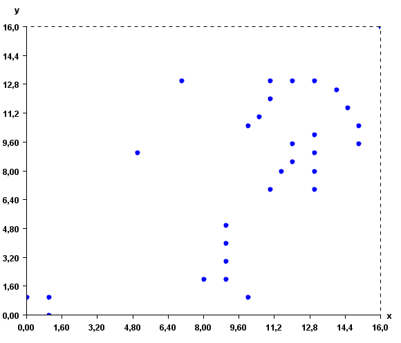
The K-Means algorithm will group the instances according to their similarity. To do this, it is also necessary to specify the distance function to be used for comparing the instances. The distance function can be the Euclidian distance, correlation
distance, cosine distance, Manathan distance and Jaccard distance. In
the command line or GUI of SPMF, the distance function is specified by
using one of these keywords: "euclidian", "correlation", "cosine",
"manathan" and "jaccard" as parameter. In this example, the euclidian distance is used.
What is the output?
K-Means groups instances in clusters according to
their similarity. In SPMF, the similarity is defined according to the
distance function chosen by the user such as the Euclidian distance. K-Means
returns K clusters or less.
Note that running K-Means with the same data
does not always generate the same result because K-Means initializes
clusters randomly.
By running K-Means on the previous input file and K=3, we can
obtain the following output file containing 3 clusters:
@ATTRIBUTEDEF=X
@ATTRIBUTEDEF=Y
[Instance12 8.0 2.0][Instance13 9.0 2.0][Instance14 10.0 1.0][Instance28 9.0 3.0][Instance29 9.0 4.0][Instance30 9.0 5.0]
[Instance4 11.0 12.0][Instance5 11.0 13.0][Instance6 13.0 13.0][Instance7 12.0 8.5][Instance8 13.0 8.0][Instance9 13.0 9.0][Instance11 11.0 7.0][Instance15 7.0 13.0][Instance16 5.0 9.0][Instance17 16.0 16.0][Instance18 11.5 8.0][Instance20 13.0 10.0][Instance21 12.0 13.0][Instance21 14.0 12.5][Instance22 14.5 11.5][Instance23 15.0 10.5][Instance24 15.0 9.5][Instance25 12.0 9.5][Instance26 10.5 11.0][Instance27 10.0 10.5][Instance10 13.0 7.0]
[Instance1 1.0 1.0][Instance2 0.0 1.0][Instance3 1.0 0.0]
The output file format is defined as follows.
The first few lines indicate the attribute names. Each attribute is specified on a separated line with the keyword "ATTRIBUTEDEF=" followed by the attribute name (a string). Then, the list of clusters is indicated. Each cluster is specified on a separated line, listing the instances contained in the cluster.
An instance is a name followed by a list of double values separated by " " and between the
"[" and "]" characters.
The clusters found by the algorithm can be viewed visually using the "Cluster Viewer" provided in SPMF. If you are using the graphical interface of SPMF, click the checkbox "Cluster Viewer" before pressing the "Run Algorithm" button. The result will be displayed in the Cluster Viewer.

As it can be seen in this example, the result somewhat make sense, as points close to each other are in the same cluster.
Applying K-Means to time series
Note that the K-Means algorithm implementation in SPMF can also be applied to time series database such as the file contextSAX.txt in the SPMF distribution. To apply K-Means to time series, it is necessary to set the "separator" parameter of the K-Means algorithm to "," since time series files separate values by "," instead of spaces.
Where can I get more information about K-Means?
K-Means was proposed by MacQueen in 1967. K-means is one of the
most famous data mining algorithm. It is described in almost all data
mining books that focus on algorithms, and on many websites. By
searching on the web, you will find plenty of resources explaining
K-Means.
Example 78 : Clustering Values with the Bisecting
K-Means algorithm
How to run this example?
- If you are using the graphical interface, (1)
choose the "BisectingKMeans"
algorithm, (2) select the input file "inputDBScan2.txt",
(3) set the output file name (e.g. "output.txt")
(4) set k =3, distance function = euclidian, iter
= 10 and(5) click "Run algorithm".
Note that there is also an optional parameter called "separator". It can be used to read other types of input files where values are not separated by spaces. For example, for a file separated by the ',' character, the parameter "separator" would have to be set to ",".
- If you want to execute this example from the command line,
then execute this command:
java -jar spmf.jar run BisectingKMeans inputDBScan2.txt
output.txt 3 euclidian 10 in a folder containing spmf.jar and the example input file inputDBScan2.txt.
- If you are using the source code version of SPMF, launch
the file "MainTestBisectingKMeans_saveToFile.java"
in the package ca.pfv.SPMF.tests.
What is Bisecting K-Means?
K-Means is one of the most famous clustering
algorithm. It is used to separate a set of instances (vectors of double values)
into groups of instances (clusters) according to their similarity.
The Bisecting K-Means algorithm is a variation
of the regular K-Means algorithm that is reported to
perform better for some applications. It consists of the following
steps: (1) pick a cluster, (2) find 2-subclusters using the basic
K-Means algorithm, * (bisecting step), (3) repeat step 2, the bisecting
step, for ITER times and take the split that produces the clustering,
(4) repeat steps 1,2,3 until the desired number of clusters is reached.
In this implementation the user can choose between various
distance functions to assess the distance between vectors. SPMF offers
the Euclidian distance, correlation distance, cosine distance, Manathan
distance and Jaccard distance.
What is the input?
Bisecting K-Means takes as input a set of
instances (each having a name and containing one or more double values), a parameter K (a positive
integer >=1) indicating the number of clusters to be created, a
distance function, and the parameter ITER.
The input file format of K-Means is a text file containing several instances.
The first lines (optional) specify the name of the attributes used for describing the instances. In this example, two attributes will be used, named X and Y. But note that more than two attributes could be used. Each attribute is specified on a separated line by the keyword "@ATTRIBUTEDEF=", followed by the attribute name
Then, each instance is described by two lines. The first line (which is optional) contains the string "@NAME=" followed by the name of the instance. Then, the second line provides a list of double values separated by single spaces.
An example of input is provided in the file "inputDBScan2.txt"
of the SPMF distribution. It contains 31 instances, each described by two attribute called X and Y.
@ATTRIBUTEDEF=X
@ATTRIBUTEDEF=Y
@NAME=Instance1
1 1
@NAME=Instance2
0 1
@NAME=Instance3
1 0
@NAME=Instance4
11 12
@NAME=Instance5
11 13
@NAME=Instance6
13 13
@NAME=Instance7
12 8.5
@NAME=Instance8
13 8
@NAME=Instance9
13 9
@NAME=Instance10
13 7
@NAME=Instance11
11 7
@NAME=Instance12
8 2
@NAME=Instance13
9 2
@NAME=Instance14
10 1
@NAME=Instance15
7 13
@NAME=Instance16
5 9
@NAME=Instance17
16 16
@NAME=Instance18
11.5 8
@NAME=Instance20
13 10
@NAME=Instance21
12 13
@NAME=Instance21
14 12.5
@NAME=Instance22
14.5 11.5
@NAME=Instance23
15 10.5
@NAME=Instance24
15 9.5
@NAME=Instance25
12 9.5
@NAME=Instance26
10.5 11
@NAME=Instance27
10 10.5
@NAME=Instance28
9 3
@NAME=Instance29
9 4
@NAME=Instance30
9 5
For example, the first instance is named "Instance1", and it is a vector with two values: 1 and 1 for the attributes X and Y, respectively.
This input file represents a set of 2D points. But note that, it is possible to use more than two attributes to describe instances. To give a better idea of what the input file looks like, here is a visual representation:
The Bisecting K-Means algorithm will group the instances according to their similarity. To do this, it is also necessary to specify the distance function to be used for comparing the instances. The distance function can be the Euclidian distance, correlation
distance, cosine distance, Manathan distance and Jaccard distance. In
the command line or GUI of SPMF, the distance function is specified by
using one of these keywords: "euclidian", "correlation", "cosine",
"manathan" and "jaccard" as parameter. In this example, the euclidian distance is used.
The ITER specifies how much times the algorithm should repeat a
split to keep the best split. If it is set to a high value it should
provide better results but it should be more slow. Splits are evaluated
using the Squared Sum of Errors (SSE).
What is the output?
Bisecting K-Means groups vectors in clusters
according to their similarity. In SPMF, the similarity is defined
according to the distance function chosen by the user such as the
Euclidian distance. K-Means returns K clusters or
less.
Note that running Bisecting K-Means with the
same data does not always generate the same result because Bisecting
K-Means initializes clusters randomly.
By running Bisecting K-Means on the previous
input file, we can
obtain the following output file containing 3 clusters:
@ATTRIBUTEDEF=X
@ATTRIBUTEDEF=Y
[Instance1 1.0 1.0][Instance2 0.0 1.0][Instance3 1.0 0.0][Instance12 8.0 2.0][Instance13 9.0 2.0][Instance14 10.0 1.0][Instance16 5.0 9.0][Instance28 9.0 3.0][Instance29 9.0 4.0][Instance30 9.0 5.0]
[Instance9 13.0 9.0][Instance24 15.0 9.5][Instance7 12.0 8.5][Instance8 13.0 8.0][Instance10 13.0 7.0][Instance11 11.0 7.0][Instance18 11.5 8.0][Instance20 13.0 10.0][Instance25 12.0 9.5][Instance23 15.0 10.5]
[Instance4 11.0 12.0][Instance5 11.0 13.0][Instance6 13.0 13.0][Instance17 16.0 16.0][Instance21 12.0 13.0][Instance21 14.0 12.5][Instance22 14.5 11.5][Instance15 7.0 13.0][Instance26 10.5 11.0][Instance27 10.0 10.5]
The output file format is defined as follows.
The first few lines indicate the attribute names. Each attribute is specified on a separated line with the keyword "ATTRIBUTEDEF=" followed by the attribute name (a string). Then, the list of clusters is indicated. Each cluster is specified on a separated line, listing the instances contained in the cluster.
An instance is a name followed by a list of double values separated by " " and between the
"[" and "]" characters.
The clusters found by the algorithm can be viewed visually using the "Cluster Viewer" provided in SPMF. If you are using the graphical interface of SPMF, click the checkbox "Cluster Viewer" before pressing the "Run Algorithm" button. The result will be displayed in the Cluster Viewer.
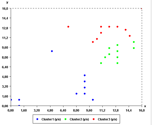
As it can be seen in this example, the result somewhat make sense, as points close to each other are in the same cluster.
Applying Bisecting K-Means to time series
Note that the Bisecting K-Means algorithm implementation in SPMF can also be applied to time series database such as the file contextSAX.txt in the SPMF distribution. To apply this algorithm to time series, it is necessary to set the "separator" parameter of this algorithm to "," since time series files separate values by "," instead of separating by spaces.
Where can I get more information about Bisecting K-Means ?
The original K-Means was proposed by MacQueen in 1967. K-means is
one of the most famous data mining algorithm. It is described in almost
all data mining books that focus on algorithms, and on many websites.
By searching on the web, you will find plenty of resources explaining
K-Means.
The Bisecting K-Means algorithms is described in this paper:
A comparison of document clustering techniques", M. Steinbach,
G. Karypis and V. Kumar. Workshop on Text Mining, KDD, 2000.
Example 79 : Clustering Values with the DBScan algorithm
How to run this example?
- If you are using the graphical interface, (1)
choose the "DBScan"
algorithm, (2) select the input file "inputDBScan2.txt",
(3) set the output file name (e.g. "output.txt")
(4) set minPts =2 and epsilon = 2, and(5) click "Run
algorithm".
Note that there is also an optional parameter called "separator". It can be used to read other types of input files where values are not separated by spaces. For example, for a file separated by the ',' character, the parameter "separator" would have to be set to ",".
- If you want to execute this example from the command line,
then execute this command:
java -jar spmf.jar run DBScan inputDBScan2.txt
output.txt 2 2 in a folder containing spmf.jar and the example input file inputDBScan2.txt.
- If you are using the source code version of SPMF, launch
the file "MainTestDBScan_saveToFile.java"
in the package ca.pfv.SPMF.tests.
What is DBScan?
DBScan is an old but famous clustering
algorithm. It is used to find clusters of points based on the density.
Implementation note: To avoid having a O(n^2) time complexity,
this implementation uses a KD-Tree to store points internally.
What is the input?
DBScan takes as input (1) a set of instances having a name and containing one or more double values, (2) a parameter minPts
(a positive integer >=1) indicating the number of points that a core
point need to have in its neighborhood (see paper about DBScan for more
details) and (3) a radius epsilon that define the
neighborhood of a point.
The input file format is is a text file containing several instances.
The first lines (optional) specify the name of the attributes used for describing the instances. In this example, two attributes will be used, named X and Y. But note that more than two attributes could be used. Each attribute is specified on a separated line by the keyword "@ATTRIBUTEDEF=", followed by the attribute name
Then, each instance is described by two lines. The first line (which is optional) contains the string "@NAME=" followed by the name of the instance. Then, the second line provides a list of double values separated by single spaces.
An example of input is provided in the file "inputDBScan2.txt"
of the SPMF distribution. It contains 31 instances, each described by two attribute called X and Y.
@ATTRIBUTEDEF=X
@ATTRIBUTEDEF=Y
@NAME=Instance1
1 1
@NAME=Instance2
0 1
@NAME=Instance3
1 0
@NAME=Instance4
11 12
@NAME=Instance5
11 13
@NAME=Instance6
13 13
@NAME=Instance7
12 8.5
@NAME=Instance8
13 8
@NAME=Instance9
13 9
@NAME=Instance10
13 7
@NAME=Instance11
11 7
@NAME=Instance12
8 2
@NAME=Instance13
9 2
@NAME=Instance14
10 1
@NAME=Instance15
7 13
@NAME=Instance16
5 9
@NAME=Instance17
16 16
@NAME=Instance18
11.5 8
@NAME=Instance20
13 10
@NAME=Instance21
12 13
@NAME=Instance21
14 12.5
@NAME=Instance22
14.5 11.5
@NAME=Instance23
15 10.5
@NAME=Instance24
15 9.5
@NAME=Instance25
12 9.5
@NAME=Instance26
10.5 11
@NAME=Instance27
10 10.5
@NAME=Instance28
9 3
@NAME=Instance29
9 4
@NAME=Instance30
9 5
For example, the first instance is named "Instance1", and it is a vector with two values: 1 and 1 for the attributes X and Y, respectively.
This input file represents a set of 2D points. But note that, it is possible to use more than two attributes to describe instances. To give a better idea of what the input file looks like, here is a visual representation:
The distance function used by Optics is the Euclidian distance
What is the output?
DBScans groups vectors (points) in clusters based
on density and distance between points.
Note that it is normal that DBScan may generate a cluster having
less than minPts (this happens if the neibhoors of a core points get
"stolen" by another cluster).
Note also that DBScan eliminate points that are seen as noise (a
point having less than minPts neighboors within a radius of epsilon)
By running DBScan on the previous input file and
minPts =2 and epsilon=2, we obtain the following output file containing
4 clusters:
@ATTRIBUTEDEF=X
@ATTRIBUTEDEF=Y
[Instance1 1.0 1.0][Instance3 1.0 0.0][Instance2 0.0 1.0]
[Instance14 10.0 1.0][Instance13 9.0 2.0][Instance28 9.0 3.0][Instance29 9.0 4.0][Instance12 8.0 2.0][Instance30 9.0 5.0]
[Instance27 10.0 10.5][Instance26 10.5 11.0][Instance4 11.0 12.0][Instance5 11.0 13.0][Instance21 12.0 13.0][Instance6 13.0 13.0][Instance21 14.0 12.5][Instance22 14.5 11.5][Instance23 15.0 10.5][Instance24 15.0 9.5]
[Instance11 11.0 7.0][Instance18 11.5 8.0][Instance7 12.0 8.5][Instance25 12.0 9.5][Instance8 13.0 8.0][Instance9 13.0 9.0][Instance10 13.0 7.0][Instance20 13.0 10.0]
The output file format is defined as follows.
The first few lines indicate the attribute names. Each attribute is specified on a separated line with the keyword "ATTRIBUTEDEF=" followed by the attribute name (a string). Then, the list of clusters is indicated. Each cluster is specified on a separated line, listing the instances contained in the cluster.
An instance is a name followed by a list of double values separated by " " and between the
"[" and "]" characters.
The clusters found by the algorithm can be viewed visually using the "Cluster Viewer" provided in SPMF. If you are using the graphical interface of SPMF, click the checkbox "Cluster Viewer" before pressing the "Run Algorithm" button. The result will be displayed in the Cluster Viewer.
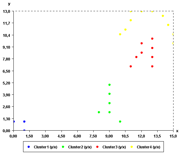
As it can be seen in this example, the result somewhat make sense. Points that are close to each other have put in the same clusters. An interesting thing about DBScan is that it can find clusters of various shapes.
Applying DBSCAN to time series
Note that the DBScan algorithm implementation in SPMF can also be applied to time series database such as the file contextSAX.txt in the SPMF distribution. To apply this algorithm to time series, it is necessary to set the "separator" parameter of this algorithm to "," since time series files separate values by "," instead of separating by spaces.
Where can I get more information about DBScan?
DBScan is a most famous data mining algorithm for clustering. It is
described in almost all data mining books that focus on algorithms, and
on many websites. The original article describing DBScan is:
Ester, Martin; Kriegel, Hans-Peter; Sander, Jörg; Xu, Xiaowei
(1996). Simoudis, Evangelos; * Han, Jiawei; Fayyad, Usama M., eds. A
density-based algorithm for discovering clusters in large spatial
databases with noise. Proceedings of the Second International
Conference on Knowledge Discovery and Data Mining (KDD-96). AAAI Press.
pp. 226–231.
Example 80 : Using Optics to extract a cluster-ordering
of points and DB-Scan style clusters
What is OPTICS?
OPTICS is a classic clustering algorithm. It
takes as input a set of instances (vectors of double values) and output a cluster-ordering of instances (points),
that is a total order on the set of instances.
This "cluster-ordering" of points can then be used to generate
density-based clusters similar to those generated by DBScan.
In the paper describing Optics, the authors also proposed authors
tasks that can be done using the cluster-ordering of points such as
interactive visualization and automatically extracting hierarchical
clusters. Those tasks are not implemented here.
Implementation note: To avoid having a O(n^2) time complexity,
this implementation uses a KD-Tree to store points internally.
In this implementation the user can choose between various
distance functions to assess the similarity between vectors. SPMF
offers the Euclidian distance, correlation distance, cosine distance,
Manathan distance and Jaccard distance.
How to run this example?
To generate a cluster-ordering of points using OPTICS:
- If you are using the graphical interface, (1)
choose the "OPTICS-cluster-ordering"
algorithm, (2) select the input file "inputDBScan2.txt",
(3) set the output file name (e.g. "output.txt")
(4) set minPts =2 and epsilon = 2, and (5) click "Run
algorithm".
Note that there is also an optional parameter called "separator". It can be used to read other types of input files where values are not separated by spaces. For example, for a file separated by the ',' character, the parameter "separator" would have to be set to ",".
- If you want to execute this example from the command line,
then execute this command:
java -jar spmf.jar run OPTICS-cluster-ordering inputDBScan2.txt
output.txt 2 2 in a folder containing spmf.jar and the example input file inputDBScan2.txt.
- If you are using the source code version of SPMF, launch
the file "MainTestOPTICS_extractClusterOrdering_saveToFile.java"
in the package ca.pfv.SPMF.tests.
To generate a DB-Scan style cluster of points using OPTICS:
- If you are using the graphical interface, (1)
choose the "OPTICS-dbscan-clusters"
algorithm, (2) select the input file "inputDBScan2.txt",
(3) set the output file name (e.g. "output.txt")
(4) set minPts =2, epsilon = 2 and epsilonPrime = 5,
and(5) click "Run algorithm".
Note that there is also an optional parameter called "separator". It can be used to read other types of input files where values are not separated by spaces. For example, for a file separated by the ',' character, the parameter "separator" would have to be set to ",".
- If you want to execute this example from the command line,
then execute this command:
java -jar spmf.jar run OPTICS-dbscan-clusters inputDBScan2.txt
output.txt 2 2 5 in a folder containing spmf.jar
and the example input file inputDBScan2.txt.
- If you are using the source code version of SPMF, launch
the file "MainTestOPTICS_extractDBScan_saveToFile.java"
in the package ca.pfv.SPMF.tests.
What is the input?
Optics takes as input (1) a set of instances (points)
having a name and containing one or more double values, (2) a parameter minPts
(a positive integer >=1) indicating the number of instances (points) that a core
point need to have in its neighborhood (see paper about Optics for more
details) and (3) a radius epsilon that define the
neighborhood of a point. If clusters are generated, an extra parameter
named epsilonPrime is also taken as parameter. This latter
parameter can be set to the same value as epsilon or a
different value (see paper for details).
The input file format is a text file containing several instances.
The first lines (optional) specify the name of the attributes used for describing the instances. In this example, two attributes will be used, named X and Y. But note that more than two attributes could be used. Each attribute is specified on a separated line by the keyword "@ATTRIBUTEDEF=", followed by the attribute name
Then, each instance is described by two lines. The first line (which is optional) contains the string "@NAME=" followed by the name of the instance. Then, the second line provides a list of double values separated by single spaces.
An example of input is provided in the file "inputDBScan2.txt"
of the SPMF distribution. It contains 31 instances, each described by two attribute called X and Y.
@ATTRIBUTEDEF=X
@ATTRIBUTEDEF=Y
@NAME=Instance1
1 1
@NAME=Instance2
0 1
@NAME=Instance3
1 0
@NAME=Instance4
11 12
@NAME=Instance5
11 13
@NAME=Instance6
13 13
@NAME=Instance7
12 8.5
@NAME=Instance8
13 8
@NAME=Instance9
13 9
@NAME=Instance10
13 7
@NAME=Instance11
11 7
@NAME=Instance12
8 2
@NAME=Instance13
9 2
@NAME=Instance14
10 1
@NAME=Instance15
7 13
@NAME=Instance16
5 9
@NAME=Instance17
16 16
@NAME=Instance18
11.5 8
@NAME=Instance20
13 10
@NAME=Instance21
12 13
@NAME=Instance21
14 12.5
@NAME=Instance22
14.5 11.5
@NAME=Instance23
15 10.5
@NAME=Instance24
15 9.5
@NAME=Instance25
12 9.5
@NAME=Instance26
10.5 11
@NAME=Instance27
10 10.5
@NAME=Instance28
9 3
@NAME=Instance29
9 4
@NAME=Instance30
9 5
For example, the first instance is named "Instance1", and it is a vector with two values: 1 and 1 for the attributes X and Y, respectively.
This input file represents a set of 2D points. But note that, it is possible to use more than two attributes to describe instances. To give a better idea of what the input file looks like, here is a visual representation:
The distance function used by Optics is the Euclidian distance
What is the output?
Optics generates a a so-called cluster-ordering
of points, which is a list of points with their reachability distances.
For example, for minPts = 2 and epsilon = 2, the following cluster
ordering is generated, where each line indicates respresent an instance (a name and its vector of values) and a
reachability distance. Note that a reachability distance equals to
"infinity" means "UNDEFINED" in the original paper.
Cluster orderings
Instance2 0.0 1.0 Infinity
Instance1 1.0 1.0 1.0
Instance3 1.0 0.0 1.0
Instance14 10.0 1.0 Infinity
Instance13 9.0 2.0 1.4142135623730951
Instance28 9.0 3.0 1.0
Instance12 8.0 2.0 1.0
Instance29 9.0 4.0 1.0
Instance30 9.0 5.0 1.0
Instance16 5.0 9.0 Infinity
Instance15 7.0 13.0 Infinity
Instance27 10.0 10.5 Infinity
Instance26 10.5 11.0 0.7071067811865476
Instance4 11.0 12.0 1.118033988749895
Instance5 11.0 13.0 1.0
Instance21 12.0 13.0 1.0
Instance6 13.0 13.0 1.0
Instance21 14.0 12.5 1.118033988749895
Instance22 14.5 11.5 1.118033988749895
Instance23 15.0 10.5 1.118033988749895
Instance24 15.0 9.5 1.0
Instance11 11.0 7.0 Infinity
Instance18 11.5 8.0 1.118033988749895
Instance7 12.0 8.5 0.7071067811865476
Instance25 12.0 9.5 1.0
Instance8 13.0 8.0 1.118033988749895
Instance9 13.0 9.0 1.0
Instance10 13.0 7.0 1.0
Instance20 13.0 10.0 1.0
Instance17 16.0 16.0 Infinity
The cluster ordering found by Optics can be used to do various
things. Among others, it can be used to generate DBScan style clusters
based on the density of points. This feature is implemented in SPMF and
is called ExtractDBScanClusters() in the original paper presenting
OPTICS. When extracting DBscan clusters it is possible to specify a
different epsilon value than the one used to extract the cluster
ordering. This new epsilon value is called "epsilonPrime" (see the
paper for details). By extracting clusters with epsilonPrime =5, we can
obtain three clusters.
@ATTRIBUTEDEF=X
@ATTRIBUTEDEF=Y
[Instance1 1.0 1.0][Instance3 1.0 0.0][Instance2 0.0 1.0]
[Instance14 10.0 1.0][Instance13 9.0 2.0][Instance28 9.0 3.0][Instance12 8.0 2.0][Instance29 9.0 4.0][Instance30 9.0 5.0]
[Instance27 10.0 10.5][Instance26 10.5 11.0][Instance4 11.0 12.0][Instance5 11.0 13.0][Instance21 12.0 13.0][Instance6 13.0 13.0][Instance21 14.0 12.5][Instance22 14.5 11.5][Instance23 15.0 10.5][Instance24 15.0 9.5]
[Instance11 11.0 7.0][Instance18 11.5 8.0][Instance7 12.0 8.5][Instance25 12.0 9.5][Instance8 13.0 8.0][Instance9 13.0 9.0][Instance10 13.0 7.0][Instance20 13.0 10.0]
The output file format is defined as follows.The output file format is defined as follows.
The first few lines indicate the attribute names. Each attribute is specified on a separated line with the keyword "ATTRIBUTEDEF=" followed by the attribute name (a string). Then, the list of clusters is indicated. Each cluster is specified on a separated line, listing the instances contained in the cluster.
An instance is a name followed by a list of double values separated by " " and between the
"[" and "]" characters.
The clusters found by the algorithm can be viewed visually using the "Cluster Viewer" provided in SPMF. If you are using the graphical interface of SPMF, click the checkbox "Cluster Viewer" before pressing the "Run Algorithm" button. The result will be displayed in the Cluster Viewer.
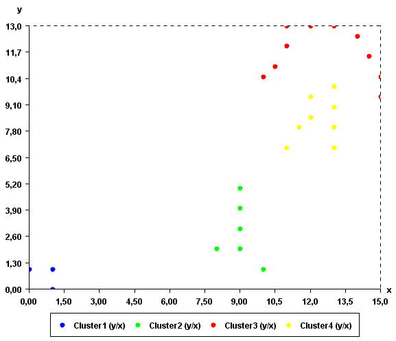
Note that it is normal that OPTICS may generate a cluster having
less than minPts in some cases. Note also that OPTICS eliminate points that are seen as noise
By running OPTICS on the previous input file and
minPts =2 and epsilon=5, we obtain the following output file containing
3 clusters:
Applying OPTICS to time series
Note that the OPTICS algorithm implementation in SPMF can also be applied to time series database such as the file contextSAX.txt in the SPMF distribution. To apply this algorithm to time series, it is necessary to set the "separator" parameter of this algorithm to "," since time series files separate values by "," instead of separating by spaces.
Where can I get more information about OPTICS?
OPTICS is a quite popular data mining algorithm. The original
paper proposing this algorithm is:
Mihael Ankerst, Markus M. Breunig, Hans-Peter Kriegel, Jörg Sander
(1999). OPTICS: Ordering Points To Identify the Clustering Structure.
ACM SIGMOD international conference on Management of data. ACM Press.
pp. 49–60.
Example 81 : Clustering Values with a Hierarchical
Clustering algorithm
How to run this example?
- If you are using the graphical interface, (1)
choose the "HierarchicalClustering"
algorithm, (2) select the input file "inputDBScan2.txt",
(3) set the output file name (e.g. "output.txt")
(4) set maxDistance to 4 (5) click "Run
algorithm".
Note that there is also an optional parameter called "separator" if you want to use other types of input files where values are not separated by spaces. For example, for a file separated by ',', the parameter "separator" would have to be set to ",".
- If you want to execute this example from the command line,
then execute this command:
java -jar spmf.jar run Hierarchical_clustering
inputDBscan2.txt output.txt 4 euclidian in a folder
containing spmf.jar and the example input
file inputDBScan2.txt.
- If you are using the source code version of SPMF, launch
the file "MainTestHierarchicalClustering.java"
in the package ca.pfv.SPMF.tests.
What is this algorithm?
We have implemented a hierarchical clustering algorithm
that is based on the description of Hierarchical Clustering Algorithms
from
http://home.dei.polimi.it/matteucc/Clustering/tutorial_html/hierarchical.html.
The algorithm is used to separate a set of instances (vectors of double values each having a name)
into groups of instances (clusters) according to their similarity. In
this implementation the euclidean distance is used to compute the
similarity.
The algorithm works as follow. It first create a cluster for each
single instance (vector). Then it recursively try to merge clusters together to
create larger clusters. To determine if two clusters can be merged, a
constant "threshold" indicate the maximal distance between two clusters
for merging.
In this implementation the user can choose between various
distance functions to assess the similarity between vectors. SPMF
offers the Euclidian distance, correlation distance, cosine distance,
Manathan distance and Jaccard distance.
What is the input?
The input is a set of instances (each having a name and containinga vector of double values),
a parameter "maxdistance" and a distance function.
The input file format is a text file containing several instances.
The first lines (optional) specify the name of the attributes used for describing the instances. In this example, two attributes will be used, named X and Y. But note that more than two attributes could be used. Each attribute is specified on a separated line by the keyword "@ATTRIBUTEDEF=", followed by the attribute name
Then, each instance is described by two lines. The first line (which is optional) contains the string "@NAME=" followed by the name of the instance. Then, the second line provides a list of double values separated by single spaces.
An example of input is provided in the file "inputDBScan2.txt"
of the SPMF distribution. It contains 31 instances, each described by two attribute called X and Y.
@ATTRIBUTEDEF=X
@ATTRIBUTEDEF=Y
@NAME=Instance1
1 1
@NAME=Instance2
0 1
@NAME=Instance3
1 0
@NAME=Instance4
11 12
@NAME=Instance5
11 13
@NAME=Instance6
13 13
@NAME=Instance7
12 8.5
@NAME=Instance8
13 8
@NAME=Instance9
13 9
@NAME=Instance10
13 7
@NAME=Instance11
11 7
@NAME=Instance12
8 2
@NAME=Instance13
9 2
@NAME=Instance14
10 1
@NAME=Instance15
7 13
@NAME=Instance16
5 9
@NAME=Instance17
16 16
@NAME=Instance18
11.5 8
@NAME=Instance20
13 10
@NAME=Instance21
12 13
@NAME=Instance21
14 12.5
@NAME=Instance22
14.5 11.5
@NAME=Instance23
15 10.5
@NAME=Instance24
15 9.5
@NAME=Instance25
12 9.5
@NAME=Instance26
10.5 11
@NAME=Instance27
10 10.5
@NAME=Instance28
9 3
@NAME=Instance29
9 4
@NAME=Instance30
9 5
For example, the first instance is named "Instance1", and it is a vector with two values: 1 and 1 for the attributes X and Y, respectively.
This input file represents a set of 2D points. But note that, it is possible to use more than two attributes to describe instances. To give a better idea of what the input file looks like, here is a visual representation:
The algorithm will group the instances according to their similarity. To do this, it is also necessary to specify the distance function to be used for comparing the instances. The distance function can be the Euclidian distance, correlation
distance, cosine distance, Manathan distance and Jaccard distance. In
the command line or GUI of SPMF, the distance function is specified by
using one of these keywords: "euclidian", "correlation", "cosine",
"manathan" and "jaccard" as parameter. In this example, the euclidian distance is used.
Furthermore, the user should also provide a parameter called maxDistance
(a positive value > 0) to the algorithm. This parameter indicate the
maximal distance allowed between the mean of two clusters to merge them
into a single cluster.
What is the output?
The algorithm groups instances in clusters according to
their similarity. In SPMF, the similarity is defined according to the
distance function chosen by the user such as the Euclidian distance.
By running the algorithm on the previous input file with maxDistance = 4 , we can
obtain the following output file containing 6 clusters:
@ATTRIBUTEDEF=X
@ATTRIBUTEDEF=Y
[Instance1 1.0 1.0][Instance2 0.0 1.0][Instance3 1.0 0.0]
[Instance4 11.0 12.0][Instance5 11.0 13.0][Instance6 13.0 13.0][Instance21 12.0 13.0][Instance26 10.5 11.0][Instance27 10.0 10.5][Instance7 12.0 8.5][Instance18 11.5 8.0][Instance8 13.0 8.0][Instance9 13.0 9.0][Instance20 13.0 10.0][Instance25 12.0 9.5][Instance10 13.0 7.0][Instance11 11.0 7.0][Instance21 14.0 12.5][Instance22 14.5 11.5][Instance23 15.0 10.5][Instance24 15.0 9.5]
[Instance12 8.0 2.0][Instance13 9.0 2.0][Instance14 10.0 1.0][Instance28 9.0 3.0][Instance29 9.0 4.0][Instance30 9.0 5.0]
[Instance15 7.0 13.0]
[Instance16 5.0 9.0]
[Instance17 16.0 16.0]
The output file format is defined as follows.
The first few lines indicate the attribute names. Each attribute is specified on a separated line with the keyword "ATTRIBUTEDEF=" followed by the attribute name (a string). Then, the list of clusters is indicated. Each cluster is specified on a separated line, listing the instances contained in the cluster.
An instance is a name followed by a list of double values separated by " " and between the
"[" and "]" characters.
The clusters found by the algorithm can be viewed visually using the "Cluster Viewer" provided in SPMF. If you are using the graphical interface of SPMF, click the checkbox "Cluster Viewer" before pressing the "Run Algorithm" button. The result will be displayed in the Cluster Viewer.
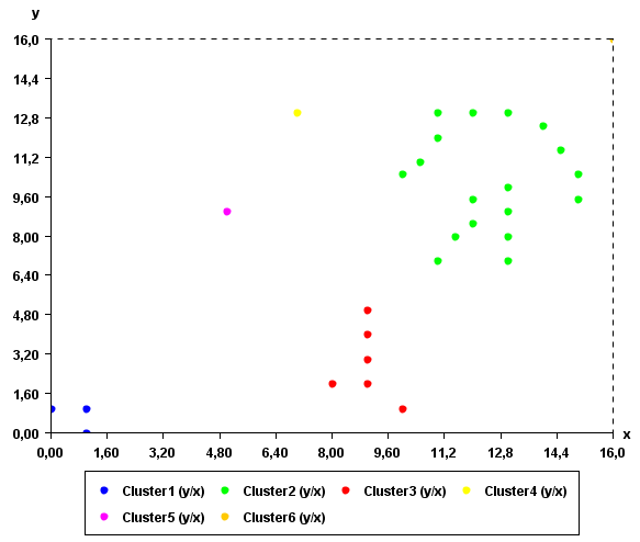
As it can be seen in this example, the result somewhat make sense. Points that are close to each other have put in the same clusters.
Applying this algorithm to time series
Note that this algorithm implementation in SPMF can also be applied to time series database such as the file contextSAX.txt in the SPMF distribution. To apply this algorithm to time series, it is necessary to set the "separator" parameter of this algorithm to "," since time series files separate values by "," instead of separating by spaces.
Where can I get more information about Hierarchical clustering?
There is a good introduction here:
http://home.dei.polimi.it/matteucc/Clustering/tutorial_html/hierarchical.html.
Moreover, you could also read the free chapter on clustering from
the book "introduction to data mining" by Tan, Steinbach and Kumar on
the book website.
Example 82 : Visualizing clusters of points using the Cluster Viewer
How to run this example?
- If you are using the graphical interface, (1)
choose the "Vizualize_clusters_of_instances" algorithm, (2) select the input file "clustersDBScan.txt", (3) and click "Run algorithm".
- If you want to execute this example from the command line,
then execute this command:
java -jar spmf.jar run Vizualize_clusters_of_instances clustersDBScan.txt
in a folder containing spmf.jar and the example input file clustersDBScan.txt.
- If you are using the source code version of SPMF, to
run respectively this example, launch
the file "MainTestClusterViewerFile.java"in
the package ca.pfv.SPMF.tests.
What is the Cluster Viewer?
The Cluster Viewer is a tool offered in SPMF for visualizing a set of clusters using a chart. The Cluster Viewer provides some basic functions like zooming in, zooming out, printing, and saving the picture as an image. It is useful for visualizing the clusters found by clustering algorithms such as DBScan, K-Means and others.
What is the input of the Cluster Viewer?
The input is one or more clusters. A cluster is a list of instances. An instance is here a list of floating-point decimal numbers (a vector of double values).
Clusters are produced by clustering algorithms such as K-Means and DBScan. An example of clusters found by the DBScan algorithm is the following:
| Cluster |
Data points |
| Cluster1 |
(1, 0), (1, 1), (0, 1) |
| Cluster2 |
(10, 10), (10, 13)(13, 13) |
| Cluster3 |
(54, 54), (57, 55) (55, 55) |
This example set of clusters is provided in the file clustersDBScan.txt of the SPMF distribution.
What is the result of running the time series viewer?
Running theCluster Viewer will display the clusters visually. For example, for the above clusters, the clusters will be displayed as follows (note that this may vary depending on your version of SPMF).
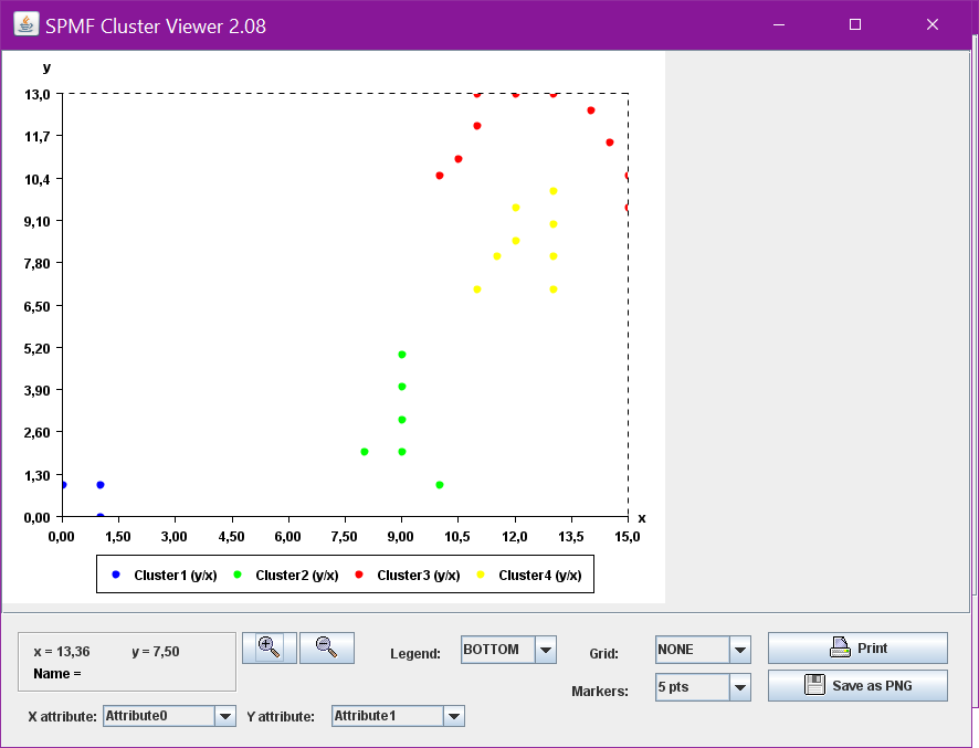
Input file format
The input file format used by the cluster viewer is defined
as follows. It is a text file.
The text file first defines the attributes used to describe the instances that have been clustered. An attribute is defined using the keyword "@ATTRIBUTEDEF=" followed by an attribute name, which is a string. Each attribute is defined on a separated line.
Then, the list of clusters is given, each cluster is specified on a separated line. For each cluster, the list of instances contained in the cluster is specified. An instance is a name followed by a list of double values separated by " " and between the "[" and "]" characters.
For instance, the input file for this example is the following:
@ATTRIBUTEDEF=X
@ATTRIBUTEDEF=Y
[Instance2 1.0 0.0][Instance0 1.0 1.0][Instance1 0.0 1.0]
[Instance3 10.0 10.0][Instance4 10.0 13.0][Instance5 13.0 13.0]
[Instance6 54.0 54.0][Instance9 57.0 55.0][Instance7 55.0 55.0]
It indicates that there are two attributes named "X" and "Y" and that there are three clusters. The first cluster contains three instances: (1, 0), (1, 1) and (0, 1).
Implementation details
The Cluster Viewer has been implemented by reusing and extending some code provided by Yuriy Guskov under the MIT License for displaying charts.
Example 83 : Visualizing instances using the Instance Viewer
How to run this example?
- If you are using the graphical interface, (1)
choose the "Vizualize_clusters_of_instances" algorithm, (2) select the input file "inputDBScan2.txt", (3) and click "Run algorithm".
- If you want to execute this example from the command line,
then execute this command:
java -jar spmf.jar run Vizualize_clusters_of_instances inputDBScan2.txt
in a folder containing spmf.jar and the example input file inputDBScan2.txt.
- If you are using the source code version of SPMF, to
run respectively this example, launch
the file "MainTestInstanceViewerFile.java"in
the package ca.pfv.SPMF.tests.
What is the Instance Viewer?
The Instance Viewer is a tool offered in SPMF for visualizing a set of instances used as input for clustering algorithms. The Instance Viewer provides some basic functions like zooming in, zooming out, printing, and saving the picture as an image. It is useful for visualizing the instances that will be given to a clustering algorithm as input. Visualizing instances can help to decide which algorithm should then be applied.
What is the input of the Instance Viewer?
The input is a file containing several instances. The input file format is defined as follows.
The first lines (optional) specify the name of the attributes used for describing the instances. In this example, two attributes will be used, named X and Y. But note that more than two attributes could be used. Each attribute is specified on a separated line by the keyword "@ATTRIBUTEDEF=", followed by the attribute name
Then, each instance is described by two lines. The first line (which is optional) contains the string "@NAME=" followed by the name of the instance. Then, the second line provides a list of double values separated by single spaces.
An example of input is provided in the file "inputDBScan2.txt"
of the SPMF distribution. It contains 31 instances, each described by two attribute called X and Y.
@ATTRIBUTEDEF=X
@ATTRIBUTEDEF=Y
@NAME=Instance1
1 1
@NAME=Instance2
0 1
@NAME=Instance3
1 0
@NAME=Instance4
11 12
@NAME=Instance5
11 13
@NAME=Instance6
13 13
@NAME=Instance7
12 8.5
@NAME=Instance8
13 8
@NAME=Instance9
13 9
@NAME=Instance10
13 7
@NAME=Instance11
11 7
@NAME=Instance12
8 2
@NAME=Instance13
9 2
@NAME=Instance14
10 1
@NAME=Instance15
7 13
@NAME=Instance16
5 9
@NAME=Instance17
16 16
@NAME=Instance18
11.5 8
@NAME=Instance20
13 10
@NAME=Instance21
12 13
@NAME=Instance21
14 12.5
@NAME=Instance22
14.5 11.5
@NAME=Instance23
15 10.5
@NAME=Instance24
15 9.5
@NAME=Instance25
12 9.5
@NAME=Instance26
10.5 11
@NAME=Instance27
10 10.5
@NAME=Instance28
9 3
@NAME=Instance29
9 4
@NAME=Instance30
9 5
For example, the first instance is named "Instance1", and it is a vector with two values: 1 and 1 for the attributes X and Y, respectively.
What is the result of running theinstance viewer?
Running the Instance Viewer will display the instances visually. For example, for the above instances, the instances will be displayed as follows (note that this may vary depending on your version of SPMF).
Implementation details
The Instance Viewer has been implemented by reusing and extending some code provided by Yuriy Guskov under the MIT License for displaying charts.
Example 84 : Mining Frequent Sequential Patterns Using the PrefixSpan Algorithm
How to run this example?
To run the implementation of PrefixSpan by P.
Fournier-Viger (PFV):
- If you are using the graphical interface, (1)
choose the "PrefixSpan"
algorithm, (2) select the input file "contextPrefixSpan.txt",
(3) set the output file name (e.g. "output.txt")
(4) set minsup = 50% and (5) click "Run
algorithm".
- If you want to execute this example from the command
line, then execute this command:
java -jar spmf.jar run PrefixSpan contextPrefixSpan.txt
output.txt 50% in a folder containing spmf.jar
and the example input file contextPrefixSpan.txt.
- If you are using the source code version of SPMF, launch
the file "MainTestPrefixSpan_saveToMemory.java"
in the package ca.pfv.SPMF.tests.
To run the version the implementation of PrefixSpan
by A. Gomariz Peñalver (AGP):
- If you are using the graphical interface, (1)
choose the "PrefixSpan_AGP"
algorithm, (2) select the input file "contextPrefixSpan.txt",
(3) set the output file name (e.g. "output.txt")
(4) set minsup = 50% and (5) click "Run
algorithm".
- If you want to execute this example from the command
line, then execute this command:
java -jar spmf.jar run PrefixSpan_AGP
contextPrefixSpan.txt output.txt 50% in a folder
containing spmf.jar and the example input
file contextPrefixSpan.txt.
- If you are using the source code version of SPMF, launch
the file "MainTestPrefixSpan_AGP_saveToMemory.java"
in the package ca.pfv.SPMF.tests
What is PrefixSpan?
PrefixSpan is an algorithm for discovering
sequential patterns in sequence databases, proposed by Pei et al.
(2001).
What is the input of PrefixSpan?
The input of PrefixSpan is a sequence database
and a user-specified threshold named minsup (a value in
[0,1] representing a percentage).
A sequence database is a set of sequences where
each sequence is a list of itemsets. An itemset is an unordered set of
distinct items. For example, the table shown below contains four
sequences. The first sequence, named S1, contains 5 itemsets. It means
that item 1 was followed by items 1 2 and 3 at the same time, which
were followed by 1 and 3, followed by 4, and followed by 3 and 6. It is
assumed that items in an itemset are sorted in lexicographical order.
This database is provided in the file "contextPrefixSpan.txt"
of the SPMF distribution. Note that it is assumed that
no items appear twice in the same itemset and that items in an itemset
are lexically ordered.
| ID |
Sequences |
| S1 |
(1), (1 2 3), (1 3), (4), (3 6) |
| S2 |
(1 4), (3), (2 3), (1 5) |
| S3 |
(5 6), (1 2), (4 6), (3), (2) |
| S4 |
(5), (7), (1 6), (3), (2), (3) |
What is the output of PrefixSpan?
PrefixSpan discovers all frequent
sequential patterns occurring in a sequence database
(subsequences that occurs in more than minsup sequences of
the database.
To explain more formally what is a sequential pattern, it is
necessary to review some definition.
A sequential pattern is a sequence. A sequence
SA = X1, X2, ... Xk, where X1, X2... Xk are itemsets
is said to occur in another sequence SB = Y1, Y2, ... Ym,
where Y1, Y2... Ym are itemsets, if and only if there exists integers 1
<= i1 < i2... < ik <= m such that X1 ⊆ Yi1, X2 ⊆ Yi2, ...
Xk ⊆ Yik.
The support of a sequential pattern is the
number of sequences where the pattern occurs divided by the total
number of sequences in the database.
A frequent sequential pattern is a sequential
pattern having a support no less than the minsup parameter
provided by the user.
For example, if we run PrefixSpan with minsup= 50 % and
with a maximum pattern length of 100 items, 53 sequential patterns are
found. The list is too long to be presented here. An example of pattern
found is "(1,2),(6)" which appears in the first and the third sequences
(it has therefore a support of 50%). This pattern has a length of 3
because it contains three items. Another pattern is "(4), (3), (2)". It
appears in the second and third sequence (it has thus a support of 50
%). It also has a length of 3 because it contains 3 items.
Optional parameter(s)
The PrefixSpan implementation allows to specify
additional optional parameter(s) :
- "maximum pattern length" allows to specify the maximum number
of items that patterns found should contain.
- "show sequences ids?" (true/false) This parameter allows to
specify that sequence ids of sequences containing a pattern should be
output for each pattern found. For example, if the parameter is set to
true, each pattern in the output file will be followed by the keyword
#SID followed by a list of sequences ids (integers separated by space).
For example, a line terminated by "#SID: 0 2" means that the pattern on
this line appears in the first and the third sequences of the sequence
database (sequences with ids 0 and 2).
These parameter(s) are available in the GUI of SPMF and also in
the example(s) "MainTestPrefixSpan ...
.java" provided in the source code of SPMF.
The parameter(s) can be also used in the command line with the Jar
file. If you want to use these optional parameter(s) in the command
line, it can be done as follows. Consider this example:
java -jar spmf.jar run PrefixSpan contextPrefixSpan.txt
output.txt 50% 5 true
This command means to apply the algorithm on the file
"contextPrefixSpan.txt" and output the results to "output.txt".
Moreover, it specifies that the user wants to find patterns for minsup
= 50%, and patterns must have a maximum length of 5 items, and sequence
ids should be output for each pattern found.
Input file format
The input file format is defined as follows. It
is a text file where each line represents a sequence from a sequence
database. Each item from a sequence is a positive integer and items
from the same itemset within a sequence are separated by single space.
Note that it is assumed that items within a same itemset are sorted
according to a total order and that no item can appear twice in the
same itemset. The value "-1" indicates the end of an itemset. The value
"-2" indicates the end of a sequence (it appears at the end of each
line). For example, the input file "contextPrefixSpan.txt" contains the
following four lines (four sequences).
1 -1 1 2 3 -1 1 3 -1 4 -1 3 6 -1 -2
1 4 -1 3 -1 2 3 -1 1 5 -1 -2
5 6 -1 1 2 -1 4 6 -1 3 -1 2 -1 -2
5 -1 7 -1 1 6 -1 3 -1 2 -1 3 -1 -2
The first line represents a sequence where the itemset {1} is
followed by the itemset {1, 2, 3}, followed by the itemset {1, 3},
followed by the itemset {4}, followed by the itemset {3, 6}. The next
lines follow the same format.
Note that it is also possible to use a text file containing a text (several sentences) if the text file has the ".text" extension, as an alternative to the default input format. If the algorithm is applied on a text file from the graphical interface or command line interface, the text file will be automatically converted to the SPMF format, by dividing the text into sentences separated by ".", "?" and "!", where each word is considered as an item. Note that when a text file is used as input of
a data mining algorithm, the performance will be slightly less than if the native
SPMF file format is used because a conversion of the input file will be
automatically performed before launching the algorithm and the result
will also have to be converted. This cost however should be small.
Output file format
The output file format is defined as follows. It
is a text file. Each line is a frequent sequential pattern. Each item
from a sequential pattern is a positive integer and items from the same
itemset within a sequence are separated by single spaces. The value
"-1" indicates the end of an itemset. On each line, the sequential
pattern is first indicated. Then, the keyword "#SUP:" appears followed
by an integer indicating the support of the pattern as a number of
sequences. For example, a few lines from the output file from the
previous example are shown below:
2 3 -1 1 -1 #SUP: 2
6 -1 2 -1 #SUP: 2
6 -1 2 -1 3 -1 #SUP: 2
The first line indicates that the frequent sequential pattern
consisting of the itemset {2, 3}, followed by the itemset {1} has a
support of 2 sequences.
Performance
PrefixSpan is one of the fastest sequential
pattern mining algorithm. However, the SPAM and SPADE implementation in
SPMF can be faster than PrefixSpan (see the "performance" section of the website for a
performance comparison).
Implementation details
Note that in the source code, we also provide examples of how to
keep the result into memory instead of saving it to a file. This can be
useful if the algorithms are integrated into another Java software.
- For the AGP version of PrefixSpan, the file MainTestPrefixSpan_AGP_saveToMemory shows how
to run the algorithm and keep the result into memory.
- For the PFV version, the file MainTestPrefixSpan_saveToMemory.java
show how to run the
algorithm to keep the result into memory.
Note also that in the source code, there is a version of
PrefixSpan based on the PFV version that takes as input a dataset with
strings instead of integers. It can be run by using the files MainTestPrefixSpan_WithStrings_saveToMemory.java
and MainTestPrefixSpanWithStrings_saveToFile.java.
For the graphical user interface version of SPMF, it is possible to use
the version of PrefixSpan that uses Strings instead of integer by
selecting "PrefixSpan with strings" and to
test it with the input file contextPrefixSpanStrings.txt.
The version of PrefixSpan with Strings was made to temporarily
accommodate the needs of some users of SPMF. In the future, it may be
replaced by a more general mechanism for using files with strings for
all algorithms.
Where can I get more information about PrefixSpan?
The PrefixSpan algorithm is described in this article:
J. Pei, J. Han, B. Mortazavi-Asl, J. Wang, H. Pinto, Q. Chen,
U. Dayal, M. Hsu: Mining
Sequential Patterns by Pattern-Growth: The PrefixSpan Approach.
IEEE Trans. Knowl. Data Eng. 16(11): 1424-1440 (2004)
Besides, you may read this survey of sequential pattern mining, which gives an overview of sequential pattern mining algorithms.
Example 85 : Mining Frequent
Sequential Patterns Using the GSP Algorithm
How to run this example?
- If you are using the graphical interface, (1)
choose the "GSP"
algorithm, (2) select the input file "contextPrefixSpan.txt",
(3) set the output file name (e.g. "output.txt")
(4) set minsup = 50%, and (5) click "Run
algorithm".
- If you want to execute this example from the command line,
then execute this command:
java -jar spmf.jar run GSP contextPrefixSpan.txt
output.txt 50% in a folder containing spmf.jar
and the example input file contextPrefixSpan.txt.
- If you are using the source code version of SPMF, launch
the file "MainTestGSP_saveToMemory.java"
in the package ca.pfv.SPMF.tests.
What is GSP?
GSP is one of the first algorithm for discovering
sequential patterns in sequence databases, proposed by Srikant et al.
(1992). It uses an Apriori-like approach for discovering sequential
patterns. Note that this version does not include the constraints
proposed in the article.
What is the input of GSP?
The input of GSP is a sequence database and a
user-specified threshold named minsup (a value in [0,1]
representing a percentage). Moreover, the implementation in SPMF adds
another parameter, which is the maximum sequential pattern length in
terms of items.
A sequence database is a set of sequences where
each sequence is a list of itemsets. An itemset is an unordered set of
distinct items. For example, the table shown below contains four
sequences. The first sequence, named S1, contains 5 itemsets. It means
that item 1 was followed by items 1 2 and 3 at the same time, which
were followed by 1 and 3, followed by 4, and followed by 3 and 6. It is
assumed that items in an itemset are sorted in lexicographical order.
This database is provided in the file "contextPrefixSpan.txt"
of the SPMF distribution. Note that it is assumed that
no items appear twice in the same itemset and that items in an itemset
are lexically ordered.
| ID |
Sequences |
| S1 |
(1), (1 2 3), (1 3), (4), (3 6) |
| S2 |
(1 4), (3), (2 3), (1 5) |
| S3 |
(5 6), (1 2), (4 6), (3), (2) |
| S4 |
(5), (7), (1 6), (3), (2), (3) |
What is the output of GSP?
GSP discovers all frequent sequential
patterns occurring in a sequence database (subsequences that
occurs in more than minsup sequences of the database.
To explain more formally what is a sequential pattern, it is
necessary to review some definition.
A sequential pattern is a sequence. A sequence
SA = X1, X2, ... Xk, where X1, X2... Xk are itemsets
is said to occur in another sequence SB = Y1, Y2, ... Ym,
where Y1, Y2... Ym are itemsets, if and only if there exists integers 1
<= i1 < i2... < ik <= m such that X1⊆Yi1, X2 ⊆ Yi2, ...
Xk ⊆ Yik.
The support of a sequential pattern is the
number of sequences where the pattern occurs divided by the total
number of sequences in the database.
A frequent sequential pattern is a sequential
pattern having a support no less than the minsup parameter
provided by the user.
For example, if we run GSP with minsup= 50 % and with a
maximum pattern length of 100 items, 53 sequential patterns are found.
The list is too long to be presented here. An example of pattern found
is "(1,2),(6)" which appears in the first and the third sequences (it
has therefore a support of 50%). This pattern has a length of 3 because
it contains three items. Another pattern is "(4), (3), (2)". It appears
in the second and third sequence (it has thus a support of 50 %). It
also has a length of 3 because it contains 3 items.
Optional parameter(s)
The GSP implementation allows to specify
additional optional parameter(s) :
- "show sequences ids?" (true/false) This parameter allows to
specify that sequence ids of sequences containing a pattern should be
output for each pattern found. For example, if the parameter is set to
true, each pattern in the output file will be followed by the keyword
#SID followed by a list of sequences ids (integers separated by space).
For example, a line terminated by "#SID: 0 2" means that the pattern on
this line appears in the first and the third sequences of the sequence
database (sequences with ids 0 and 2).
These parameter(s) are available in the GUI of SPMF and also in
the example(s) "MainTestGSP ... .java"
provided in the source code of SPMF.
The parameter(s) can be also used in the command line with the Jar
file. If you want to use these optional parameter(s) in the command
line, it can be done as follows. Consider this example:
java -jar spmf.jar run GSP contextPrefixSpan.txt
output.txt 50% 5 true
This command means to apply the algorithm on the file
"contextPrefixSpan.txt" and output the results to "output.txt".
Moreover, it specifies that the user wants to find patterns for minsup
= 50%, and sequence ids should be output for each pattern found
Input file format
The input file format is defined as follows. It
is a text file where each line represents a sequence from a sequence
database. Each item from a sequence is a positive integer and items
from the same itemset within a sequence are separated by single space.
Note that it is assumed that items within a same itemset are sorted
according to a total order and that no item can appear twice in the
same itemset. The value "-1" indicates the end of an itemset. The value
"-2" indicates the end of a sequence (it appears at the end of each
line). For example, the input file "contextPrefixSpan.txt" contains the
following four lines (four sequences).
1 -1 1 2 3 -1 1 3 -1 4 -1 3 6 -1 -2
1 4 -1 3 -1 2 3 -1 1 5 -1 -2
5 6 -1 1 2 -1 4 6 -1 3 -1 2 -1 -2
5 -1 7 -1 1 6 -1 3 -1 2 -1 3 -1 -2
The first line represents a sequence where the itemset {1} is
followed by the itemset {1, 2, 3}, followed by the itemset {1, 3},
followed by the itemset {4}, followed by the itemset {3, 6}. The next
lines follow the same format.
Note that it is also possible to use a text file containing a text (several sentences) if the text file has the ".text" extension, as an alternative to the default input format. If the algorithm is applied on a text file from the graphical interface or command line interface, the text file will be automatically converted to the SPMF format, by dividing the text into sentences separated by ".", "?" and "!", where each word is considered as an item. Note that when a text file is used as input of
a data mining algorithm, the performance will be slightly less than if the native
SPMF file format is used because a conversion of the input file will be
automatically performed before launching the algorithm and the result
will also have to be converted. This cost however should be small.
Output file format
The output file format is defined as follows. It
is a text file. Each line is a frequent sequential pattern. Each item
from a sequential pattern is a positive integer and items from the same
itemset within a sequence are separated by single spaces. The value
"-1" indicates the end of an itemset. On each line, the sequential
pattern is first indicated. Then, the keyword " #SUP: " appears
followed by an integer indicating the support of the pattern as a
number of sequences. For example, a few lines from the output file from
the previous example are shown below:
2 3 -1 1 -1 #SUP: 2
6 -1 2 -1 #SUP: 2
6 -1 2 -1 3 -1 #SUP: 2
The first line indicates that the frequent sequential pattern
consisting of the itemset {2, 3}, followed by the itemset {1} has a
support of 2 sequences. The next lines follow the same format.
Performance
See the "performance" section of the
website for a performance comparison with other sequential pattern
mining algorithm.
Implementation details
The implementation is faithful to the article, except that the gap
constraints and window constraints are currently not implemented (will
be considered in future versions of SPMF).
Also note that in the source code, we also provide an example of
how to run GSP and keep the result into memory instead of saving it to
a file ("MainTestGSP_saveToMemory.java".).
This can be useful if the algorithms are integrated into another Java
software.
Where can I get more information about GSP?
The GSP algorithm is described in this article:
R. Srikant and R. Agrawal. 1996. Mining Sequential Patterns: Generalizations and
Performance Improvements. In Proceedings of the 5th International
Conference on Extending Database Technology: Advances in Database
Technology (EDBT '96), Peter M. G. Apers, Mokrane Bouzeghoub, and
Georges Gardarin (Eds.). Springer-Verlag, London, UK, UK, 3-17.
Besides, you may read this survey of sequential pattern mining, which gives an overview of sequential pattern mining algorithms.
Example 86: Mining Frequent Sequential Patterns Using the SPADE Algorithm
How to run this example?
- If you are using the graphical interface, (1)
choose the "SPADE"
algorithm, (2) select the input file "contextPrefixSpan.txt",
(3) set the output file name (e.g. "output.txt")
(4) set minsup = 50% and (5) click "Run
algorithm".
- If you want to execute this example from the command
line, then execute this command:
java -jar spmf.jar run SPADE contextPrefixSpan.txt
output.txt 50% in a folder containing spmf.jar
and the example input file contextPrefixSpan.txt.
- If you are using the source code version of SPMF, launch
the file "MainTestSPADE_AGP_FatBitMap_saveToFile.java"
in the package ca.pfv.SPMF.tests
What is SPADE?
SPADE is a popular sequential pattern mining
algorithm proposed by Zaki
What is the input of SPADE?
The input of SPADE is a sequence database and
a user-specified threshold named minsup (a value in [0,1]
representing a percentage). Moreover, the implementation in SPMF adds
another parameter, which is the maximum sequential pattern length in
terms of items.
A sequence database is a set of sequences
where each sequence is a list of itemsets. An itemset is an unordered
set of distinct items. For example, the table shown below contains four
sequences. The first sequence, named S1, contains 5 itemsets. It means
that item 1 was followed by items 1 2 and 3 at the same time, which
were followed by 1 and 3, followed by 4, and followed by 3 and 6. It is
assumed that items in an itemset are sorted in lexicographical order.
This database is provided in the file "contextPrefixSpan.txt"
of the SPMF distribution. Note that it is assumed that
no items appear twice in the same itemset and that items in an itemset
are lexically ordered.
| ID |
Sequences |
| S1 |
(1), (1 2 3), (1 3), (4), (3 6) |
| S2 |
(1 4), (3), (2 3), (1 5) |
| S3 |
(5 6), (1 2), (4 6), (3), (2) |
| S4 |
(5), (7), (1 6), (3), (2), (3) |
What is the output of SPADE?
SPADE discovers all frequent
sequential patterns occurring in a sequence database
(subsequences that occurs in more than minsup sequences of
the database.
To explain more formally what is a sequential pattern, it is
necessary to review some definition.
A sequential pattern is a sequence. A sequence
SA = X1, X2, ... Xk, where X1, X2... Xk are
itemsets is said to occur in another sequence SB = Y1,
Y2, ... Ym, where Y1, Y2... Ym are itemsets, if and only if there
exists integers 1 <= i1 < i2... < ik <= m such that X1 ⊆
Yi1, X2 ⊆ Yi2, ... Xk ⊆ Yik.
The support of a sequential pattern is the
number of sequences where the pattern occurs divided by the total
number of sequences in the database.
A frequent sequential pattern is a sequential
pattern having a support no less than the minsup parameter
provided by the user.
For example, if we run SPADE with minsup= 50 % and
with a maximum pattern length of 100 items, 53 sequential patterns are
found. The list is too long to be presented here. An example of pattern
found is "(1,2),(6)" which appears in the first and the third sequences
(it has therefore a support of 50%). This pattern has a length of 3
because it contains three items. Another pattern is "(4), (3), (2)". It
appears in the second and third sequence (it has thus a support of 50
%). It also has a length of 3 because it contains 3 items.
Optional parameter(s)
The SPADE implementation allows to specify
additional optional parameter(s) :
- "show sequences ids?" (true/false) This parameter allows to
specify that sequence ids of sequences containing a pattern should be
output for each pattern found. For example, if the parameter is set to
true, each pattern in the output file will be followed by the keyword
#SID followed by a list of sequences ids (integers separated by space).
For example, a line terminated by "#SID: 1 3" means that the pattern on
this line appears in the first and the third sequences of the sequence
database.
These parameter(s) are available in the GUI of SPMF and also in
the example(s) "MainTestSPADE ... .java"
provided in the source code of SPMF.
The parameter(s) can be also used in the command line with the
Jar file. If you want to use these optional parameter(s) in the command
line, it can be done as follows. Consider this example:
java -jar spmf.jar run SPADE contextPrefixSpan.txt
output.txt 50% true
This command means to apply the algorithm on the file
"contextPrefixSpan.txt" and output the results to "output.txt".
Moreover, it specifies that the user wants to find patterns for minsup
= 50%, and sequence ids should be output for each pattern found.
Input file format
The input file format is defined as follows.
It is a text file where each line represents a sequence from a sequence
database. Each item from a sequence is a positive integer and items
from the same itemset within a sequence are separated by single space.
Note that it is assumed that items within a same itemset are sorted
according to a total order and that no item can appear twice in the
same itemset. The value "-1" indicates the end of an itemset. The value
"-2" indicates the end of a sequence (it appears at the end of each
line). For example, the input file "contextPrefixSpan.txt" contains the
following four lines (four sequences).
1 -1 1 2 3 -1 1 3 -1 4 -1 3 6 -1 -2
1 4 -1 3 -1 2 3 -1 1 5 -1 -2
5 6 -1 1 2 -1 4 6 -1 3 -1 2 -1 -2
5 -1 7 -1 1 6 -1 3 -1 2 -1 3 -1 -2
The first line represents a sequence where the itemset {1} is
followed by the itemset {1, 2, 3}, followed by the itemset {1, 3},
followed by the itemset {4}, followed by the itemset {3, 6}. The next
lines follow the same format.
Note that it is also possible to use a text file containing a text (several sentences) if the text file has the ".text" extension, as an alternative to the default input format. If the algorithm is applied on a text file from the graphical interface or command line interface, the text file will be automatically converted to the SPMF format, by dividing the text into sentences separated by ".", "?" and "!", where each word is considered as an item. Note that when a text file is used as input of
a data mining algorithm, the performance will be slightly less than if the native
SPMF file format is used because a conversion of the input file will be
automatically performed before launching the algorithm and the result
will also have to be converted. This cost however should be small.
Output file format
The output file format is defined as follows.
It is a text file. Each line is a frequent sequential pattern. Each
item from a sequential pattern is a positive integer and items from the
same itemset within a sequence are separated by single spaces. The
value "-1" indicates the end of an itemset. On each line, the
sequential pattern is first indicated. Then, the keyword " #SUP: "
appears followed by an integer indicating the support of the pattern as
a number of sequences. For example, a few lines from the output file
from the previous example are shown below:
2 3 -1 1 -1 #SUP: 2
6 -1 2 -1 #SUP: 2
6 -1 2 -1 3 -1 #SUP: 2
The first line indicates that the frequent sequential pattern
consisting of the itemset {2, 3}, followed by the itemset {1} has a
support of 2 sequences. The next lines follow the same format.
Performance
See the "performance" section of
the website for a performance comparison with other sequential pattern
mining algorithm.
Implementation details
In the source code, we also provide examples of how to keep the
result into memory instead of saving it to a file. This can be useful
if the algorithms are integrated into another Java software. Examples
of how to save result into memory are named according to the following
naming convention: "MainTest..._saveToMemory".
Also note that in the source code, there are three variations
the SPADE implementations that tries different ways to perform the join
of IdLists. The fastest implementation is the one named "Fat_Bitmap".
It is the one offered in the graphical user interface.
"MainTestSPADE_AGP_BitMap_saveToFile.java"
"MainTestSPADE_AGP_BitMap_saveToMemory.java"
"MainTestSPADE_AGP_EntryList_saveToFile.java"
"MainTestSPADE_AGP_EntryList_saveToMemory.java"
"MainTestSPADE_AGP_FatBitMap_saveToFile.java"
"MainTestSPADE_AGP_FatBitMap_saveToMemory.java"
Lastly, in the source code, a parallelized version of SPADE is
also offered:
"MainTestSPADE_AGP_Parallelized_BitMap_saveToFile.java"
"MainTestSPADE_AGP_Parallelized_BitMap_saveToMemory.java"
"MainTestSPADE_AGP_Parallelized_EntryList_saveToFile.java"
"MainTestSPADE_AGP_Parallelized_EntryList_saveToMemory.java"
"MainTestSPADE_AGP_Parallelized_FatBitMap_saveToFile.java"
"MainTestSPADE_AGP_Parallelized_FatBitMap_saveToMemory.java"
Besides, note that an alternative input file contextSPADE.txt is provided. It contains the
example used in the article proposing SPADE.
Where can I get more information about SPADE?
The SPADE algorithm is described in this article:
Mohammed J. Zaki. 2001. SPADE:
An Efficient Algorithm for Mining Frequent Sequences. Mach. Learn.
42, 1-2 (January 2001), 31-60. DOI=10.1023/A:1007652502315
http://dx.doi.org/10.1023/A:1007652502315
Besides, you may read this survey of sequential pattern mining, which gives an overview of sequential pattern mining algorithms.
Example 87: Mining Frequent Sequential Patterns Using the CM-SPADE Algorithm
How to run this example?
- If you are using the graphical interface, (1)
choose the "CM-SPADE"
algorithm, (2) select the input file "contextPrefixSpan.txt",
(3) set the output file name (e.g. "output.txt")
(4) set minsup = 50% and (5) click "Run
algorithm".
- If you want to execute this example from the command
line, then execute this command:
java -jar spmf.jar run CM-SPADE contextPrefixSpan.txt
output.txt 50% in a folder containing spmf.jar
and the example input file contextPrefixSpan.txt.
- If you are using the source code version of SPMF, launch
the file "MainTestCMSPADE_saveToFile.java"
in the package ca.pfv.SPMF.tests
What is CM-SPADE?
CM-SPADE is a sequential pattern mining
algorithm based on the SPADE algorithm.
The main difference is that CM-SPADE utilizes a new technique
named co-occurrence pruning to prune the search space, which makes
faster.
What is the input of CM-SPADE?
The input of CM-SPADE is a sequence database
and a user-specified threshold named minsup (a value in
[0,1] representing a percentage). Moreover, the implementation in SPMF
adds another parameter, which is the maximum sequential pattern length
in terms of items.
A sequence database is a set of sequences
where each sequence is a list of itemsets. An itemset is an unordered
set of distinct items. For example, the table shown below contains four
sequences. The first sequence, named S1, contains 5 itemsets. It means
that item 1 was followed by items 1 2 and 3 at the same time, which
were followed by 1 and 3, followed by 4, and followed by 3 and 6. It is
assumed that items in an itemset are sorted in lexicographical order.
This database is provided in the file "contextPrefixSpan.txt"
of the SPMF distribution. Note that it is assumed that
no items appear twice in the same itemset and that items in an itemset
are lexically ordered.
| ID |
Sequences |
| S1 |
(1), (1 2 3), (1 3), (4), (3 6) |
| S2 |
(1 4), (3), (2 3), (1 5) |
| S3 |
(5 6), (1 2), (4 6), (3), (2) |
| S4 |
(5), (7), (1 6), (3), (2), (3) |
What is the output of CM-SPADE?
CM-SPADE discovers all frequent
sequential patterns occurring in a sequence database
(subsequences that occurs in more than minsup sequences of
the database.
To explain more formally what is a sequential pattern, it is
necessary to review some definition.
A sequential pattern is a sequence. A sequence
SA = X1, X2, ... Xk, where X1, X2... Xk are
itemsets is said to occur in another sequence SB = Y1,
Y2, ... Ym, where Y1, Y2... Ym are itemsets, if and only if there
exists integers 1 <= i1 < i2... < ik <= m such that X1 ⊆
Yi1, X2 ⊆ Yi2, ... Xk ⊆ Yik.
The support of a sequential pattern is the
number of sequences where the pattern occurs divided by the total
number of sequences in the database.
A frequent sequential pattern is a sequential
pattern having a support no less than the minsup parameter
provided by the user.
For example, if we run CM-SPADE with minsup= 50 % and
with a maximum pattern length of 100 items, 53 sequential patterns are
found. The list is too long to be presented here. An example of pattern
found is "(1,2),(6)" which appears in the first and the third sequences
(it has therefore a support of 50%). This pattern has a length of 3
because it contains three items. Another pattern is "(4), (3), (2)". It
appears in the second and third sequence (it has thus a support of 50
%). It also has a length of 3 because it contains 3 items.
Optional parameter(s)
The CM-SPADE implementation allows to specify
additional optional parameter(s) :
- "show sequences ids?" (true/false) This parameter allows to
specify that sequence ids of sequences containing a pattern should be
output for each pattern found. For example, if the parameter is set to
true, each pattern in the output file will be followed by the keyword
#SID followed by a list of sequences ids (integers separated by space).
For example, a line terminated by "#SID: 1 3" means that the pattern on
this line appears in the first and the third sequences of the sequence
database.
These parameter(s) are available in the GUI of SPMF and also in
the example(s) "MainTestCMSpade ... .java"
provided in the source code of SPMF.
The parameter(s) can be also used in the command line with the
Jar file. If you want to use these optional parameter(s) in the command
line, it can be done as follows. Consider this example:
java -jar spmf.jar run CM-SPADE contextPrefixSpan.txt
output.txt 50% true
This command means to apply the algorithm on the file
"contextPrefixSpan.txt" and output the results to "output.txt".
Moreover, it specifies that the user wants to find patterns for minsup
= 50%, and sequence ids should be output for each pattern found.
Input file format
The input file format is defined as follows.
It is a text file where each line represents a sequence from a sequence
database. Each item from a sequence is a positive integer and items
from the same itemset within a sequence are separated by single space.
Note that it is assumed that items within a same itemset are sorted
according to a total order and that no item can appear twice in the
same itemset. The value "-1" indicates the end of an itemset. The value
"-2" indicates the end of a sequence (it appears at the end of each
line). For example, the input file "contextPrefixSpan.txt" contains the
following four lines (four sequences).
1 -1 1 2 3 -1 1 3 -1 4 -1 3 6 -1 -2
1 4 -1 3 -1 2 3 -1 1 5 -1 -2
5 6 -1 1 2 -1 4 6 -1 3 -1 2 -1 -2
5 -1 7 -1 1 6 -1 3 -1 2 -1 3 -1 -2
The first line represents a sequence where the itemset {1} is
followed by the itemset {1, 2, 3}, followed by the itemset {1, 3},
followed by the itemset {4}, followed by the itemset {3, 6}. The next
lines follow the same format.
Note that it is also possible to use a text file containing a text (several sentences) if the text file has the ".text" extension, as an alternative to the default input format. If the algorithm is applied on a text file from the graphical interface or command line interface, the text file will be automatically converted to the SPMF format, by dividing the text into sentences separated by ".", "?" and "!", where each word is considered as an item. Note that when a text file is used as input of
a data mining algorithm, the performance will be slightly less than if the native
SPMF file format is used because a conversion of the input file will be
automatically performed before launching the algorithm and the result
will also have to be converted. This cost however should be small.
Output file format
The output file format is defined as follows.
It is a text file. Each line is a frequent sequential pattern. Each
item from a sequential pattern is a positive integer and items from the
same itemset within a sequence are separated by single spaces. The
value "-1" indicates the end of an itemset. On each line, the
sequential pattern is first indicated. Then, the keyword " #SUP: "
appears followed by an integer indicating the support of the pattern as
a number of sequences. For example, a few lines from the output file
from the previous example are shown below:
2 3 -1 1 -1 #SUP: 2
6 -1 2 -1 #SUP: 2
6 -1 2 -1 3 -1 #SUP: 2
The first line indicates that the frequent sequential pattern
consisting of the itemset {2, 3}, followed by the itemset {1} has a
support of 2 sequences. The next lines follow the same format.
Performance
CM-SPADE is faster than SPADE and also the best sequential
pattern mining algorithm in SPMF according to our experiment in the
CM-SPADE paper.
Implementation details
In the source code, we also provide examples of how to keep the
result into memory instead of saving it to a file. This can be useful
if the algorithms are integrated into another Java software. Examples
of how to save result into memory is found in the following file: "MainTestCMSPADE_saveToMemory".
Where can I get more information about CM-SPADE?
The CM-SPADE algorithm is described in this article:
Fournier-Viger, P., Gomariz, A., Campos, M., Thomas, R.
(2014). Fast
Vertical Mining of Sequential Patterns Using Co-occurrence Information.
Proc. 18th Pacific-Asia Conference on Knowledge Discovery and Data
Mining (PAKDD 2014), Part 1, Springer, LNAI, 8443. pp. 40-52.
Besides, you may read this survey of sequential pattern mining, which gives an overview of sequential pattern mining algorithms.
Example 88: Mining Frequent Sequential Patterns Using the SPAM Algorithm
How to run this example?
To run the implementation of SPAM by P.
Fournier-Viger (PFV):
- If you are using the graphical interface, (1)
choose the "SPAM"
algorithm, (2) select the input file "contextPrefixSpan.txt",
(3) set the output file name (e.g. "output.txt")
(4) set minsup = 50% and maximum pattern length = 100, (5)
click "Run algorithm".
- If you want to execute this example from the command
line, then execute this command:
java -jar spmf.jar run SPAM contextPrefixSpan.txt
output.txt 50% 100 in a folder containing spmf.jar
and the example input file contextPrefixSpan.txt.
- If you are using the source code version of SPMF, launch
the file "MainTestSPAM.java"
in the package ca.pfv.SPMF.tests.
To run the version the implementation of SPAM by
A. Gomariz Peñalver (AGP):
- If you are using the graphical interface, (1)
choose the "SPAM_AGP"
algorithm, (2) select the input file "contextPrefixSpan.txt",
(3) set the output file name (e.g. "output.txt")
(4) set minsup = 50% and (5) click "Run algorithm".
- If you want to execute this example from the command
line, then execute this command:
java -jar spmf.jar run SPAM_AGP contextPrefixSpan.txt
output.txt 50% in a folder containing spmf.jar
and the example input file contextPrefixSpan.txt.
- If you are using the source code version of SPMF, launch
the file "MainTestSPAM_AGP_FatBitMap_saveToFile.java"
in the package ca.pfv.SPMF.tests.
(other variations are also available in the source code)
What is SPAM?
SPAM is an algorithm for discovering frequent
sequential patterns in a sequence database. It was proposed by Ayres
(2002).
What is the input of SPAM?
The input of SPAM is a sequence database and a
user-specified threshold named minsup (a value in [0,1]
representing a percentage). Moreover, the implementation in SPMF adds
another parameter, which is the maximum sequential pattern length in
terms of items.
A sequence database is a set of sequences where
each sequence is a list of itemsets. An itemset is an unordered set of
items. For example, the table shown below contains four sequences. The
first sequence, named S1, contains 5 itemsets. It means that item 1 was
followed by items 1 2 and 3 at the same time, which were followed by 1
and 3, followed by 4, and followed by 3 and 6. It is assumed that items
in an itemset are sorted in lexicographical order. This database is
provided in the file "contextPrefixSpan.txt" of the
SPMF distribution. Note that it is assumed that no
items appear twice in the same itemset and that items in an itemset are
lexically ordered.
| ID |
Sequences |
| S1 |
(1), (1 2 3), (1 3), (4), (3 6) |
| S2 |
(1 4), (3), (2 3), (1 5) |
| S3 |
(5 6), (1 2), (4 6), (3), (2) |
| S4 |
(5), (7), (1 6), (3), (2), (3) |
What is the output of SPAM?
SPAM discovers all frequent sequential
patterns occurring in a sequence database (subsequences that
occurs in more than minsup sequences of the database.
To explain more formally what is a sequential pattern, it is
necessary to review some definition.
A sequential pattern is a sequence. A sequence
SA = X1, X2, ... Xk, where X1, X2... Xk are itemsets
is said to occur in another sequence SB = Y1, Y2, ... Ym,
where Y1, Y2... Ym are itemsets, if and only if there exists integers 1
<= i1 < i2... < ik <= m such that X1 ⊆ Yi1, X2 ⊆ Yi2, ...
Xk ⊆ Yik.
The support of a sequential pattern is the
number of sequences where the pattern occurs divided by the total
number of sequences in the database.
A frequent sequential pattern is a sequential
pattern having a support no less than the minsup parameter
provided by the user.
For example, if we run SPAM with minsup= 50 %, 53
sequential patterns will be found. The list is too long to be presented
here. An example of pattern found is "(1,2),(6)" which appears in the
first and the third sequences (it has therefore a support of 50%). This
pattern has a length of 3 because it contains three items. Another
pattern is "(4), (3), (2)". It appears in the second and third sequence
(it has thus a support of 50 %). It also has a length of 3 because it
contains 3 items.
Optional parameters
The SPAM implementation allows to specify four optional parameters
:
- "minimum pattern length" allows to specify the minimum number
of items that patterns found should contain.
- "maximum pattern length" allows to specify the maximum number
of items that patterns found should contain.
- "max gap" allows to specify if gaps are allowed in sequential
patterns. For example, if "max gap" is set to 1, no gap is allowed
(i.e. each consecutive itemset of a pattern must appear consecutively
in a sequence). If "max gap" is set to N, a gap of N-1 itemsets is
allowed between two consecutive itemsets of a pattern. If the parameter
is not used, by default "max gap" is set to +∞.
- "show sequences ids?" (true/false) This parameter allows to
specify that sequence ids of sequences containing a pattern should be
output for each pattern found. For example, if the parameter is set to
true, each pattern in the output file will be followed by the keyword
#SID followed by a list of sequences ids (integers separated by space).
For example, a line terminated by "#SID: 0 2" means that the pattern on
this line appears in the first and the third sequences of the sequence
database (sequences with ids 0 and 2).
These parameters are available in the GUI of SPMF and also in the
example "MainTestSPAM.java"
provided in the source code of SPMF.
The parameter(s) can be also used in the command line with the Jar
file. If you want to use these optional parameters in the command line,
it can be done as follows. Consider this example:
java -jar spmf.jar run SPAM contextPrefixSpan.txt
output.txt 0.5 2 6 1 true
This command means to apply SPAM on the file
"contextPrefixSpan.txt" and output the results to "output.txt".
Moreover, it specifies that the user wants to find patterns for minsup
= 0.5, that patterns must have a minimum length of 2 items, a maximum
length of 6 items, and have no gap between itemsets, and that ids of
sequence where the patterns is found must be shown in the output.
Input file format
The input file format is defined as follows. It
is a text file where each line represents a sequence from a sequence
database. Each item from a sequence is a positive integer and items
from the same itemset within a sequence are separated by single space.
Note that it is assumed that items within a same itemset are sorted
according to a total order and that no item can appear twice in the
same itemset. The value "-1" indicates the end of an itemset. The value
"-2" indicates the end of a sequence (it appears at the end of each
line). For example, the input file "contextPrefixSpan.txt" contains the
following four lines (four sequences).
1 -1 1 2 3 -1 1 3 -1 4 -1 3 6 -1 -2
1 4 -1 3 -1 2 3 -1 1 5 -1 -2
5 6 -1 1 2 -1 4 6 -1 3 -1 2 -1 -2
5 -1 7 -1 1 6 -1 3 -1 2 -1 3 -1 -2
The first line represents a sequence where the itemset {1} is
followed by the itemset {1, 2, 3}, followed by the itemset {1, 3},
followed by the itemset {4}, followed by the itemset {3, 6}. The next
lines follow the same format.
Note that it is also possible to use a text file containing a text (several sentences) if the text file has the ".text" extension, as an alternative to the default input format. If the algorithm is applied on a text file from the graphical interface or command line interface, the text file will be automatically converted to the SPMF format, by dividing the text into sentences separated by ".", "?" and "!", where each word is considered as an item. Note that when a text file is used as input of
a data mining algorithm, the performance will be slightly less than if the native
SPMF file format is used because a conversion of the input file will be
automatically performed before launching the algorithm and the result
will also have to be converted. This cost however should be small.
Output file format
The output file format is defined as follows. It
is a text file. Each line is a frequent sequential pattern. Each item
from a sequential pattern is a positive integer and items from the same
itemset within a sequence are separated by single spaces. The value
"-1" indicates the end of an itemset. On each line, the sequential
pattern is first indicated. Then, the keyword " #SUP: " appears
followed by an integer indicating the support of the pattern as a
number of sequences. For example, a few lines from the output file from
the previous example are shown below:
2 3 -1 1 -1 #SUP: 2
6 -1 2 -1 #SUP: 2
6 -1 2 -1 3 -1 #SUP: 2
The first line indicates that the frequent sequential pattern
consisting of the itemset {2, 3}, followed by the itemset {1} has a
support of 2 sequences. The next lines follow the same format.
Performance
SPAM is one of the fastest sequential pattern
mining algorithm. The SPAM implementation in SPMF is reported to be
faster than PrefixSpan (see the "performance" section
of the website for a performance comparison). However, CM-SPAM
is faster than SPAM.
Implementation details
In the source code, we also provide examples of how to keep the
result into memory instead of saving it to a file. This can be useful
if the algorithms are integrated into another Java software. Examples
of how to save result into memory are named according to the following
naming convention: "MainTest..._saveToMemory".
For the AGP implementation of SPAM, several version are provided
in the source code that shows different way to perform the join of
IdLists. The fastest implementation is the one named "Fat_Bitmap". It
is the one offered in the graphical user interface.
- MainTestSPAM_AGP_BitMap_saveToFile.java"
- "MainTestSPAM_AGP_BitMap_saveToMemory.java"
- "MainTestSPAM_AGP_EntryList_saveToFile.java"
- "MainTestSPAM_AGP_EntryList_saveToMemory.java"
- "MainTestSPAM_AGP_FatBitMap_saveToFile.java"
- "MainTestSPAM_AGP_FatBitMap_saveToMemory.java"
The AGP and PFV implementations of SPAM shares some source code
but also have some significant differences. See the performance section of the website for a
performance comparison (will be added at the end of August 2013).
Where can I get more information about SPAM?
The SPAM algorithm was proposed in this paper:
J. Ayres, J. Gehrke, T.Yiu, and J. Flannick. Sequential
Pattern Mining Using Bitmaps. In Proceedings of the Eighth ACM
SIGKDD International Conference on Knowledge Discovery and Data Mining.
Edmonton, Alberta, Canada, July 2002.
The implementation of the optional "maxgap" constraint is based on
this paper:
Ho, J., Lukov, L., & Chawla, S. (2005). Sequential pattern
mining with constraints on large protein databases. In Proceedings
of the 12th International Conference on Management of Data
(COMAD) (pp. 89-100).
Besides, you may read this survey of sequential pattern mining, which gives an overview of sequential pattern mining algorithms.
Example 89: Mining Frequent Sequential Patterns Using the CM-SPAM Algorithm
How to run this example?
- If you are using the graphical interface, (1)
choose the "CM-SPAM"
algorithm, (2) select the input file "contextPrefixSpan.txt",
(3) set the output file name (e.g. "output.txt")
(4) set minsup = 50% and (5) click "Run algorithm".
- If you want to execute this example from the command line,
then execute this command:
java -jar spmf.jar run CMSPAM contextPrefixSpan.txt
output.txt 50% in a folder containing spmf.jar
and the example input file contextPrefixSpan.txt.
- If you are using the source code version of SPMF, launch
the file "MainTestCMSPAM_saveToFile.java"
in the package ca.pfv.SPMF.tests.
What is CMSPAM?
CM-SPAM (2013) is a sequential pattern mining
algorithm based on the SPAM algorithm.
The main difference is that CM-SPAM utilizes a new technique named
co-occurrence pruning to prune the search space, which makes it faster
than the original SPAM algorithm.
What is the input of CM-SPAM?
The input of CM-SPAM is a sequence database and
a user-specified threshold named minsup (a value in [0,1]
representing a percentage). Moreover, the implementation in SPMF adds
another parameter, which is the maximum sequential pattern length in
terms of items.
A sequence database is a set of sequences where
each sequence is a list of itemsets. An itemset is an unordered set of
items. For example, the table shown below contains four sequences. The
first sequence, named S1, contains 5 itemsets. It means that item 1 was
followed by items 1 2 and 3 at the same time, which were followed by 1
and 3, followed by 4, and followed by 3 and 6. It is assumed that items
in an itemset are sorted in lexicographical order. This database is
provided in the file "contextPrefixSpan.txt" of the
SPMF distribution. Note that it is assumed that no
items appear twice in the same itemset and that items in an itemset are
lexically ordered.
| ID |
Sequences |
| S1 |
(1), (1 2 3), (1 3), (4), (3 6) |
| S2 |
(1 4), (3), (2 3), (1 5) |
| S3 |
(5 6), (1 2), (4 6), (3), (2) |
| S4 |
(5), (7), (1 6), (3), (2), (3) |
What is the output of CM-SPAM?
CM-SPAM discovers all frequent
sequential patterns occurring in a sequence database
(subsequences that occurs in more than minsup sequences of
the database.
To explain more formally what is a sequential pattern, it is
necessary to review some definition.
A sequential pattern is a sequence. A sequence
SA = X1, X2, ... Xk, where X1, X2... Xk are itemsets
is said to occur in another sequence SB = Y1, Y2, ... Ym,
where Y1, Y2... Ym are itemsets, if and only if there exists integers 1
<= i1 < i2... < ik <= m such that X1 ⊆ Yi1, X2 ⊆ Yi2, ...
Xk ⊆ Yik.
The support of a sequential pattern is the
number of sequences where the pattern occurs divided by the total
number of sequences in the database.
A frequent sequential pattern is a sequential
pattern having a support no less than the minsup parameter
provided by the user.
For example, if we run CM-SPAM with minsup= 50 %, 53
sequential patterns will be found. The list is too long to be presented
here. An example of pattern found is "(1,2),(6)" which appears in the
first and the third sequences (it has therefore a support of 50%). This
pattern has a length of 3 because it contains three items. Another
pattern is "(4), (3), (2)". It appears in the second and third sequence
(it has thus a support of 50 %). It also has a length of 3 because it
contains 3 items.
Optional parameters
The CM-SPAM implementation allows to specify additional optional
parameter(s) :
- "minimum pattern length" allows to specify the minimum number
of items that patterns found should contain.
- "maximum pattern length" allows to specify the maximum number
of items that patterns found should contain.
- "required items" allow to specify a set of items that must
appears in every patterns found.
- "max gap" allows to specify if gaps are allowed in sequential
patterns. For example, if "max gap" is set to 1, no gap is allowed
(i.e. each consecutive itemset of a pattern must appear consecutively
in a sequence). If "max gap" is set to N, a gap of N-1 itemsets is
allowed between two consecutive itemsets of a pattern. If the parameter
is not used, by default "max gap" is set to +∞.
- "show sequences ids?" (true/false) This parameter allows to
specify that sequence ids of sequences containing a pattern should be
output for each pattern found. For example, if the parameter is set to
true, each pattern in the output file will be followed by the keyword
#SID followed by a list of sequences ids (integers separated by space).
For example, a line terminated by "#SID: 0 2" means that the pattern on
this line appears in the first and the third sequences of the sequence
database (sequences with ids 0 and 2).
These parameters are available in the GUI of SPMF and also in the
example "MainTestCMSPAM.java"
provided in the source code of SPMF.
The parameter(s) can be also used in the command line with the Jar
file. If you want to use these optional parameters in the command line,
it can be done as follows. Consider this example:
java -jar spmf.jar run CM-SPAM contextPrefixSpan.txt
output.txt 0.5 2 6 1,3 1 true
This command means to apply CM-SPAM on the file
"contextPrefixSpan.txt" and output the results to "output.txt".
Moreover, it specifies that the user wants to find patterns for minsup
= 0.5, and patterns must have a minimum length of 2 items, a maximum
length of 6 items, must contain items 2 and 3, and have no gap between
itemsets. Moreover, sequence ids should be output for each pattern
found.
Now, let's say that you want to run the algorithm again with the same parameters except that you don't want to use the "required items" parameter. You could do as follows:
java -jar spmf.jar run CM-SPAM contextPrefixSpan.txt
output.txt 0.5 2 6 "" 1 true
Input file format
The input file format is defined as follows. It
is a text file where each line represents a sequence from a sequence
database. Each item from a sequence is a positive integer and items
from the same itemset within a sequence are separated by single space.
Note that it is assumed that items within a same itemset are sorted
according to a total order and that no item can appear twice in the
same itemset. The value "-1" indicates the end of an itemset. The value
"-2" indicates the end of a sequence (it appears at the end of each
line). For example, the input file "contextPrefixSpan.txt" contains the
following four lines (four sequences).
1 -1 1 2 3 -1 1 3 -1 4 -1 3 6 -1 -2
1 4 -1 3 -1 2 3 -1 1 5 -1 -2
5 6 -1 1 2 -1 4 6 -1 3 -1 2 -1 -2
5 -1 7 -1 1 6 -1 3 -1 2 -1 3 -1 -2
The first line represents a sequence where the itemset {1} is
followed by the itemset {1, 2, 3}, followed by the itemset {1, 3},
followed by the itemset {4}, followed by the itemset {3, 6}. The next
lines follow the same format.
Note that it is also possible to use a text file containing a text (several sentences) if the text file has the ".text" extension, as an alternative to the default input format. If the algorithm is applied on a text file from the graphical interface or command line interface, the text file will be automatically converted to the SPMF format, by dividing the text into sentences separated by ".", "?" and "!", where each word is considered as an item. Note that when a text file is used as input of
a data mining algorithm, the performance will be slightly less than if the native
SPMF file format is used because a conversion of the input file will be
automatically performed before launching the algorithm and the result
will also have to be converted. This cost however should be small.
Output file format
The output file format is defined as follows. It
is a text file. Each line is a frequent sequential pattern. Each item
from a sequential pattern is a positive integer and items from the same
itemset within a sequence are separated by single spaces. The value
"-1" indicates the end of an itemset. On each line, the sequential
pattern is first indicated. Then, the keyword " #SUP: " appears
followed by an integer indicating the support of the pattern as a
number of sequences. For example, a few lines from the output file from
the previous example are shown below:
2 3 -1 1 -1 #SUP: 2
6 -1 2 -1 #SUP: 2
6 -1 2 -1 3 -1 #SUP: 2
The first line indicates that the frequent sequential pattern
consisting of the itemset {2, 3}, followed by the itemset {1} has a
support of 2 sequences. The next lines follow the same format.
Performance
CM-SPAM is faster than SPAM and
one of the best sequential pattern mining algorithm in SPMF according
to our experiment in the CM-SPAM paper (see Performance section of the
website for more details).
Where can I get more information about CM-SPAM?
The CM-SPAM algorithm is described in this article:
Fournier-Viger, P., Gomariz, A., Campos, M., Thomas, R.
(2014). Fast
Vertical Mining of Sequential Patterns Using Co-occurrence Information.
Proc. 18th Pacific-Asia Conference on Knowledge Discovery and Data
Mining (PAKDD 2014), Part 1, Springer, LNAI, 8443. pp. 40-52.
Besides, you may read this survey of sequential pattern mining, which gives an overview of sequential pattern mining algorithms.
Example 90: Mining Frequent Sequential Patterns Using the LAPIN Algorithm
How to run this example?
- If you are using the graphical interface, (1)
choose the "LAPIN"
algorithm, (2) select the input file "contextPrefixSpan.txt",
(3) set the output file name (e.g. "output.txt")
(4) set minsup = 50% and (5) click "Run algorithm".
- If you want to execute this example from the command line,
then execute this command:
java -jar spmf.jar run LAPIN contextPrefixSpan.txt
output.txt 50% in a folder containing spmf.jar
and the example input file contextPrefixSpan.txt.
- If you are using the source code version of SPMF, launch
the file "MainTestLAPIN_saveToFile.java"
in the package ca.pfv.SPMF.tests.
What is LAPIN?
LAPIN (2005) is a sequential pattern mining
algorithm based on the SPAM algorithm. It replaces join operations by
border calculations (which are similar to a projected database) and
uses a table called "Item-is-exist-table" to know if an item can appear
after a given position in a sequence. There are several variations of
LAPIN. In this implementation, we have followed the main one also known
as LAPIN, LAPIN-SPAM and LAPIN-LCI, depending on the paper where it is
described by the authors.
What is the input of LAPIN?
The input of LAPIN is a sequence database and a
user-specified threshold named minsup (a value in [0,1]
representing a percentage). Moreover, the implementation in SPMF adds
another parameter, which is the maximum sequential pattern length in
terms of items.
A sequence database is a set of sequences where
each sequence is a list of itemsets. An itemset is an unordered set of
items. For example, the table shown below contains four sequences. The
first sequence, named S1, contains 5 itemsets. It means that item 1 was
followed by items 1 2 and 3 at the same time, which were followed by 1
and 3, followed by 4, and followed by 3 and 6. It is assumed that items
in an itemset are sorted in lexicographical order. This database is
provided in the file "contextPrefixSpan.txt" of the
SPMF distribution. Note that it is assumed that no
items appear twice in the same itemset and that items in an itemset are
lexically ordered.
| ID |
Sequences |
| S1 |
(1), (1 2 3), (1 3), (4), (3 6) |
| S2 |
(1 4), (3), (2 3), (1 5) |
| S3 |
(5 6), (1 2), (4 6), (3), (2) |
| S4 |
(5), (7), (1 6), (3), (2), (3) |
What is the output of LAPIN?
LAPIN discovers all frequent sequential
patterns occurring in a sequence database (subsequences that
occurs in more than minsup sequences of the database.
To explain more formally what is a sequential pattern, it is
necessary to review some definition.
A sequential pattern is a sequence. A sequence
SA = X1, X2, ... Xk, where X1, X2... Xk are itemsets
is said to occur in another sequence SB = Y1, Y2, ... Ym,
where Y1, Y2... Ym are itemsets, if and only if there exists integers 1
<= i1 < i2... < ik <= m such that X1 ⊆ Yi1, X2 ⊆ Yi2, ...
Xk ⊆ Yik.
The support of a sequential pattern is the
number of sequences where the pattern occurs divided by the total
number of sequences in the database.
A frequent sequential pattern is a sequential
pattern having a support no less than the minsup parameter
provided by the user.
For example, if we run LAPIN with minsup= 50 %, 53
sequential patterns will be found. The list is too long to be presented
here. An example of pattern found is "(1,2),(6)" which appears in the
first and the third sequences (it has therefore a support of 50%). This
pattern has a length of 3 because it contains three items. Another
pattern is "(4), (3), (2)". It appears in the second and third sequence
(it has thus a support of 50 %). It also has a length of 3 because it
contains 3 items.
Input file format
The input file format is defined as follows. It
is a text file where each line represents a sequence from a sequence
database. Each item from a sequence is a positive integer and items
from the same itemset within a sequence are separated by single space.
Note that it is assumed that items within a same itemset are sorted
according to a total order and that no item can appear twice in the
same itemset. The value "-1" indicates the end of an itemset. The value
"-2" indicates the end of a sequence (it appears at the end of each
line). For example, the input file "contextPrefixSpan.txt" contains the
following four lines (four sequences).
1 -1 1 2 3 -1 1 3 -1 4 -1 3 6 -1 -2
1 4 -1 3 -1 2 3 -1 1 5 -1 -2
5 6 -1 1 2 -1 4 6 -1 3 -1 2 -1 -2
5 -1 7 -1 1 6 -1 3 -1 2 -1 3 -1 -2
The first line represents a sequence where the itemset {1} is
followed by the itemset {1, 2, 3}, followed by the itemset {1, 3},
followed by the itemset {4}, followed by the itemset {3, 6}. The next
lines follow the same format.
Note that it is also possible to use a text file containing a text (several sentences) if the text file has the ".text" extension, as an alternative to the default input format. If the algorithm is applied on a text file from the graphical interface or command line interface, the text file will be automatically converted to the SPMF format, by dividing the text into sentences separated by ".", "?" and "!", where each word is considered as an item. Note that when a text file is used as input of
a data mining algorithm, the performance will be slightly less than if the native
SPMF file format is used because a conversion of the input file will be
automatically performed before launching the algorithm and the result
will also have to be converted. This cost however should be small.
Output file format
The output file format is defined as follows. It
is a text file. Each line is a frequent sequential pattern. Each item
from a sequential pattern is a positive integer and items from the same
itemset within a sequence are separated by single spaces. The value
"-1" indicates the end of an itemset. On each line, the sequential
pattern is first indicated. Then, the keyword " #SUP: " appears
followed by an integer indicating the support of the pattern as a
number of sequences. For example, a few lines from the output file from
the previous example are shown below:
2 3 -1 1 -1 #SUP: 2
6 -1 2 -1 #SUP: 2
6 -1 2 -1 3 -1 #SUP: 2
The first line indicates that the frequent sequential pattern
consisting of the itemset {2, 3}, followed by the itemset {1} has a
support of 2 sequences. The next lines follow the same format.
Performance
LAPIN is quite a fast algorithm. However, it is
most of the times slower than CM-SPADE and CM-SPAM on the datasets that
we have compared. The implementation is quite optimized. Perhaps that
additional optimizations could be found to improve the speed further.
Where can I get more information about LAPIN?
The LAPIN algorithm is described in this article:
Z. Yang, Y. Wang, and M. Kitsuregawa. LAPIN: Effective Sequential Pattern Mining Algorithms
by Last Position Induction. Technical Report, Info. and Comm. Eng.
Dept., Tokyo University, 2005.
Besides, you may read this survey of sequential pattern mining, which gives an overview of sequential pattern mining algorithms.
Example 91 : Mining Frequent Closed Sequential Patterns
Using the ClaSP Algorithm
How to run this example?
- If you are using the graphical interface, (1)
choose the "ClaSP"
algorithm, (2) select the input file "contextPrefixSpan.txt",
(3) set the output file name (e.g. "output.txt")
(4) set minsup = 50% and (5) click "Run
algorithm".
- If you want to execute this example from the command line,
then execute this command:
java -jar spmf.jar run ClaSP contextPrefixSpan.txt
output.txt 50% in a folder containing spmf.jar
and the example input file contextPrefixSpan.txt.
- If you are using the source code version of SPMF, launch
the file "MainTestClaSP_saveToFile.java"
in the package ca.pfv.SPMF.tests.
What is ClaSP?
ClaSP is a very efficient algorithm for
discovering closed sequential patterns in sequence databases, proposed
by Antonio Gomariz Peñalver et al. (2013). This implementation is the
original implementation.
What is the input of ClaSP?
The input of ClaSP is a sequence database and a
user-specified threshold named minsup (a value in [0,1]
representing a percentage).
A sequence database is a set of sequences where
each sequence is a list of itemsets. An itemset is an unordered set of
items. For example, the table shown below contains four sequences. The
first sequence, named S1, contains 5 itemsets. It means that item 1 was
followed by items 1 2 and 3 at the same time, which were followed by 1
and 3, followed by 4, and followed by 3 and 6. It is assumed that items
in an itemset are sorted in lexicographical order. This database is
provided in the file "contextPrefixSpan.txt" of the
SPMF distribution. Note that it is assumed that no
items appear twice in the same itemset and that items in an itemset are
lexically ordered.
| ID |
Sequences |
| S1 |
(1), (1 2 3), (1 3), (4), (3 6) |
| S2 |
(1 4), (3), (2 3), (1 5) |
| S3 |
(5 6), (1 2), (4 6), (3), (2) |
| S4 |
(5), (7), (1 6), (3), (2), (3) |
What is the output of ClaSP?
ClaSP discovers all frequent closed
sequential patterns that occurs in a sequence database.
To explain more formally what is a closed sequential pattern, it
is necessary to review some definition.
A sequential pattern is a sequence. A sequence
SA = X1, X2, ... Xk, where X1, X2... Xk are itemsets
is said to occur in another sequence SB = Y1, Y2, ... Ym,
where Y1, Y2... Ym are itemsets, if and only if there exists integers 1
<= i1 < i2... < ik <= m such that X1 ⊆ Yi1, X2 ⊆ Yi2, ...
Xk ⊆ Yik.
The support of a sequential pattern is the
number of sequences where the pattern occurs divided by the total
number of sequences in the database.
A frequent sequential pattern is a sequential
pattern having a support no less than the minsup parameter
provided by the user.
A closed sequential pattern is a sequential
pattern such that it is not strictly included in another pattern having
the same support.
Why using ClaSP? It can be shown that the set of
closed sequential patterns is generally much smaller than the set of
sequential patterns and that no information small. Moreover, finding
closed sequential patterns is often much more efficient than
discovering all patterns.
For example, if we run ClaSP with
minsup= 50 % on the sequence database, the following
patterns are found.
| ID |
Closed Sequential Pattern |
Support |
| S1 |
(6) |
75 % |
| S2 |
(5) |
75 % |
| S3 |
(2), (3) |
75 % |
| S4 |
(1), (2) |
100 % |
| S5 |
(1), (3) |
100 % |
| S6 |
(1 2), (6) |
50 % |
| S7 |
(4), (3) |
75 % |
| S8 |
(1) (2), (3) |
50 % |
| S9 |
(1), (2 3), (1) |
50 % |
| S10 |
(1), (3), (2) |
75 % |
| S11 |
(1), (3), (3) |
75 % |
| S12 |
(1 2), (4), (3) |
50 % |
| S13 |
(6), (2), (3) |
50 % |
| S14 |
(5), (2), (3) |
50 % |
| S15 |
(4), (3), (2) |
50 % |
| S16 |
(5), (6), (3), (2) |
50 % |
| S17 |
(5), (1), (3), (2) |
50 % |
For instance, the sequential pattern "(1,2),(6)" appears in the
first and third sequence (it has therefore a support of 50%). Another
pattern is "(4), (3)". It appears in the second and third sequence (it
has thus a support of 75 %).
Optional parameter(s)
The ClaSP implementation allows to specify
additional optional parameter(s) :
- "show sequences ids?" (true/false) This parameter allows to
specify that sequence ids of sequences containing a pattern should be
output for each pattern found. For example, if the parameter is set to
true, each pattern in the output file will be followed by the keyword
#SID followed by a list of sequences ids (integers separated by space).
For example, a line terminated by "#SID: 1 3" means that the pattern on
this line appears in the first and the third sequences of the sequence
database.
These parameter(s) are available in the GUI of SPMF and also in
the example(s) "MainTestClaSP ... .java"
provided in the source code of SPMF.
The parameter(s) can be also used in the command line with the Jar
file. If you want to use these optional parameter(s) in the command
line, it can be done as follows. Consider this example:
java -jar spmf.jar run ClaSP contextPrefixSpan.txt
output.txt 50% true
This command means to apply the algorithm on the file
"contextPrefixSpan.txt" and output the results to "output.txt".
Moreover, it specifies that the user wants to find patterns for minsup
= 50%, and sequence ids should be output for each pattern found.
Input file format
The input file format is defined as follows. It
is a text file where each line represents a sequence from a sequence
database. Each item from a sequence is a positive integer and items
from the same itemset within a sequence are separated by single space.
Note that it is assumed that items within a same itemset are sorted
according to a total order and that no item can appear twice in the
same itemset. The value "-1" indicates the end of an itemset. The value
"-2" indicates the end of a sequence (it appears at the end of each
line). For example, the input file "contextPrefixSpan.txt" contains the
following four lines (four sequences).
1 -1 1 2 3 -1 1 3 -1 4 -1 3 6 -1 -2
1 4 -1 3 -1 2 3 -1 1 5 -1 -2
5 6 -1 1 2 -1 4 6 -1 3 -1 2 -1 -2
5 -1 7 -1 1 6 -1 3 -1 2 -1 3 -1 -2
The first line represents a sequence where the itemset {1} is
followed by the itemset {1, 2, 3}, followed by the itemset {1, 3},
followed by the itemset {4}, followed by the itemset {3, 6}. The next
lines follow the same format.
Note that it is also possible to use a text file containing a text (several sentences) if the text file has the ".text" extension, as an alternative to the default input format. If the algorithm is applied on a text file from the graphical interface or command line interface, the text file will be automatically converted to the SPMF format, by dividing the text into sentences separated by ".", "?" and "!", where each word is considered as an item. Note that when a text file is used as input of
a data mining algorithm, the performance will be slightly less than if the native
SPMF file format is used because a conversion of the input file will be
automatically performed before launching the algorithm and the result
will also have to be converted. This cost however should be small.
Output file format
The output file format is defined as follows. It
is a text file. Each line is a frequent sequential pattern. Each item
from a sequential pattern is a positive integer and items from the same
itemset within a sequence are separated by single spaces. The value
"-1" indicates the end of an itemset. On each line, the sequential
pattern is first indicated. Then, the keyword " #SUP: " appears
followed by an integer indicating the support of the pattern as a
number of sequences. For example, a few lines from the output file from
the previous example are shown below:
1 2 -1 4 -1 3 -1 #SUP: 2
1 2 -1 6 -1 #SUP: 2
1 -1 2 -1 3 -1 #SUP: 2
The first line indicates that the frequent sequential pattern
consisting of the itemset {1, 2}, followed by the itemset {4}, followed
by the itemset {3} has a support of 2 sequences. The next lines follow
the same format.
Performance
ClaSP is a very efficient algorithm for closed
sequential pattern mining. See the article proposing ClaSP
for a performance comparison with CloSpan and SPADE. Note that CM-ClaSP
is generally faster than ClaSP.
Implementation details
In the source code
version of SPMF, there is also an example of how to use ClaSP and keep
the result in memory instead of saving it to a file ( MainTestClaSP_saveToMemory.java ).
An alternative input file contextClaSP.txt
is also provided. It contains the example sequence database used in the
article proposing ClaSP.
Where can I get more information about this algorithm?
The ClaSP algorithm was proposed in this paper:
A. Gomariz, M. Campos, R. Marín and B. Goethals (2013), ClaSP: An
Efficient Algorithm for Mining Frequent Closed Sequences. Proc. PAKDD
2013, pp. 50-61.
Besides, you may read this survey of sequential pattern mining, which gives an overview of sequential pattern mining algorithms.
Example 92 : Mining Frequent Closed
Sequential Patterns Using the CM-ClaSP Algorithm
How to run this example?
- If you are using the graphical interface, (1)
choose the "CM-ClaSP"
algorithm, (2) select the input file "contextPrefixSpan.txt",
(3) set the output file name (e.g. "output.txt")
(4) set minsup = 50% and (5) click "Run
algorithm".
- If you want to execute this example from the command line,
then execute this command:
java -jar spmf.jar run CM-ClaSP contextPrefixSpan.txt
output.txt 50% in a folder containing spmf.jar
and the example input file contextPrefixSpan.txt.
- If you are using the source code version of SPMF, launch
the file "MainTestCMClaSP_saveToFile.java"
in the package ca.pfv.SPMF.tests.
What is CM-ClaSP?
ClaSP is a very efficient algorithm for
discovering closed sequential patterns in sequence databases, proposed
(Gomariz et al, 2013).
CM-ClaSP is a modification of the original ClaSP
algorithm using a technique co-occurrence pruning to prune the search
space (Fournier-Viger, Gomariz et al., 2014). It is generally faster
than the original ClaSP.
What is the input of CM-ClaSP?
The input of CM-ClaSP is a sequence database
and a user-specified threshold named minsup (a value in [0,1]
representing a percentage).
A sequence database is a set of sequences where
each sequence is a list of itemsets. An itemset is an unordered set of
items. For example, the table shown below contains four sequences. The
first sequence, named S1, contains 5 itemsets. It means that item 1 was
followed by items 1 2 and 3 at the same time, which were followed by 1
and 3, followed by 4, and followed by 3 and 6. It is assumed that items
in an itemset are sorted in lexicographical order. This database is
provided in the file "contextPrefixSpan.txt" of the
SPMF distribution. Note that it is assumed that no
items appear twice in the same itemset and that items in an itemset are
lexically ordered.
| ID |
Sequences |
| S1 |
(1), (1 2 3), (1 3), (4), (3 6) |
| S2 |
(1 4), (3), (2 3), (1 5) |
| S3 |
(5 6), (1 2), (4 6), (3), (2) |
| S4 |
(5), (7), (1 6), (3), (2), (3) |
What is the output of CM-ClaSP?
CM-ClaSP discovers all frequent closed
sequential patterns that occurs in a sequence database.
To explain more formally what is a closed sequential pattern, it
is necessary to review some definition.
A sequential pattern is a sequence. A sequence
SA = X1, X2, ... Xk, where X1, X2... Xk are itemsets
is said to occur in another sequence SB = Y1, Y2, ... Ym,
where Y1, Y2... Ym are itemsets, if and only if there exists integers 1
<= i1 < i2... < ik <= m such that X1 ⊆ Yi1, X2 ⊆ Yi2, ...
Xk ⊆ Yik.
The support of a sequential pattern is the
number of sequences where the pattern occurs divided by the total
number of sequences in the database.
A frequent sequential pattern is a sequential
pattern having a support no less than the minsup parameter
provided by the user.
A closed sequential pattern is a sequential
pattern such that it is not strictly included in another pattern having
the same support.
Why using CM-ClaSP? It can be shown that the set
of closed sequential patterns is generally much smaller than the set of
sequential patterns and that no information small. Moreover, finding
closed sequential patterns is often much more efficient than
discovering all patterns.
For example, if we run CM-ClaSP with
minsup= 50 % on the sequence database, the following
patterns are found.
| ID |
Closed Sequential Pattern |
Support |
| S1 |
(6) |
75 % |
| S2 |
(5) |
75 % |
| S3 |
(2), (3) |
75 % |
| S4 |
(1), (2) |
100 % |
| S5 |
(1), (3) |
100 % |
| S6 |
(1 2), (6) |
50 % |
| S7 |
(4), (3) |
75 % |
| S8 |
(1) (2), (3) |
50 % |
| S9 |
(1), (2 3), (1) |
50 % |
| S10 |
(1), (3), (2) |
75 % |
| S11 |
(1), (3), (3) |
75 % |
| S12 |
(1 2), (4), (3) |
50 % |
| S13 |
(6), (2), (3) |
50 % |
| S14 |
(5), (2), (3) |
50 % |
| S15 |
(4), (3), (2) |
50 % |
| S16 |
(5), (6), (3), (2) |
50 % |
| S17 |
(5), (1), (3), (2) |
50 % |
For instance, the sequential pattern "(1,2),(6)" appears in the
first and third sequence (it has therefore a support of 50%). Another
pattern is "(4), (3)". It appears in the second and third sequence (it
has thus a support of 75 %).
Optional parameter(s)
The CM-ClaSP implementation allows to specify
additional optional parameter(s) :
- "show sequences ids?" (true/false) This parameter allows to
specify that sequence ids of sequences containing a pattern should be
output for each pattern found. For example, if the parameter is set to
true, each pattern in the output file will be followed by the keyword
#SID followed by a list of sequences ids (integers separated by space).
For example, a line terminated by "#SID: 1 3" means that the pattern on
this line appears in the first and the third sequences of the sequence
database.
These parameter(s) are available in the GUI of SPMF and also in
the example(s) "MainTestCMClaSP ... .java"
provided in the source code of SPMF.
The parameter(s) can be also used in the command line with the Jar
file. If you want to use these optional parameter(s) in the command
line, it can be done as follows. Consider this example:
java -jar spmf.jar run CM-ClaSP contextPrefixSpan.txt
output.txt 50% true
This command means to apply the algorithm on the file
"contextPrefixSpan.txt" and output the results to "output.txt".
Moreover, it specifies that the user wants to find patterns for minsup
= 50%, and sequence ids should be output for each pattern found.
Input file format
The input file format is defined as follows. It
is a text file where each line represents a sequence from a sequence
database. Each item from a sequence is a positive integer and items
from the same itemset within a sequence are separated by single space.
Note that it is assumed that items within a same itemset are sorted
according to a total order and that no item can appear twice in the
same itemset. The value "-1" indicates the end of an itemset. The value
"-2" indicates the end of a sequence (it appears at the end of each
line). For example, the input file "contextPrefixSpan.txt" contains the
following four lines (four sequences).
1 -1 1 2 3 -1 1 3 -1 4 -1 3 6 -1 -2
1 4 -1 3 -1 2 3 -1 1 5 -1 -2
5 6 -1 1 2 -1 4 6 -1 3 -1 2 -1 -2
5 -1 7 -1 1 6 -1 3 -1 2 -1 3 -1 -2
The first line represents a sequence where the itemset {1} is
followed by the itemset {1, 2, 3}, followed by the itemset {1, 3},
followed by the itemset {4}, followed by the itemset {3, 6}. The next
lines follow the same format.
Note that it is also possible to use a text file containing a text (several sentences) if the text file has the ".text" extension, as an alternative to the default input format. If the algorithm is applied on a text file from the graphical interface or command line interface, the text file will be automatically converted to the SPMF format, by dividing the text into sentences separated by ".", "?" and "!", where each word is considered as an item. Note that when a text file is used as input of
a data mining algorithm, the performance will be slightly less than if the native
SPMF file format is used because a conversion of the input file will be
automatically performed before launching the algorithm and the result
will also have to be converted. This cost however should be small.
Output file format
The output file format is defined as follows. It
is a text file. Each line is a frequent sequential pattern. Each item
from a sequential pattern is a positive integer and items from the same
itemset within a sequence are separated by single spaces. The value
"-1" indicates the end of an itemset. On each line, the sequential
pattern is first indicated. Then, the keyword " #SUP: " appears
followed by an integer indicating the support of the pattern as a
number of sequences. For example, a few lines from the output file from
the previous example are shown below:
1 2 -1 4 -1 3 -1 #SUP: 2
1 2 -1 6 -1 #SUP: 2
1 -1 2 -1 3 -1 #SUP: 2
The first line indicates that the frequent sequential pattern
consisting of the itemset {1, 2}, followed by the itemset {4}, followed
by the itemset {3} has a support of 2 sequences. The next lines follow
the same format.
Performance
ClaSP is a very efficient algorithm for closed
sequential pattern mining. CM-ClaSP is generally a few times faster
than ClaSP on most dataset (see the CM-ClaSP paper
for details).
Implementation details
In the source code
version of SPMF, there is also an example of how to use CM-ClaSP and
keep the result in memory instead of saving it to a file (
MainTestCMClaSP_saveToMemory.java ).
Where can I get more information about this algorithm?
The CM-ClaSP algorithm was proposed in this
paper:
Fournier-Viger, P., Gomariz, A., Campos, M., Thomas, R. (2014). Fast
Vertical Mining of Sequential Patterns Using Co-occurrence Information.
Proc. 18th Pacific-Asia Conference on Knowledge Discovery and Data
Mining (PAKDD 2014), Part 1, Springer, LNAI, 8443. pp. 40-52.
Besides, you may read this survey of sequential pattern mining, which gives an overview of sequential pattern mining algorithms.
Example 93 : Mining Frequent Closed
Sequential Patterns Using the CloSpan Algorithm
How to run this example?
- If you are using the graphical interface, (1)
choose the "CloSpan"
algorithm, (2) select the input file "contextPrefixSpan.txt",
(3) set the output file name (e.g. "output.txt")
(4) set minsup = 50% and (5) click "Run
algorithm".
- If you want to execute this example from the command line,
then execute this command:
java -jar spmf.jar run CloSpan contextPrefixSpan.txt
output.txt 50% in a folder containing spmf.jar
and the example input file contextPrefixSpan.txt.
- If you are using the source code version of SPMF, launch
the file "MainTestCloSpan_saveToFile.java"
in the package ca.pfv.SPMF.tests.
What is CloSpan?
CloSpan is a pattern-growth algorithm for
discovering closed sequential patterns in sequence databases, proposed
by Yan et al. (2003),
What is the input of CloSpan?
The input of CloSpan is a sequence database and
a user-specified threshold named minsup (a value in [0,1]
representing a percentage).
A sequence database is a set of sequences where
each sequence is a list of itemsets. An itemset is an unordered set of
items. For example, the table shown below contains four sequences. The
first sequence, named S1, contains 5 itemsets. It means that item 1 was
followed by items 1 2 and 3 at the same time, which were followed by 1
and 3, followed by 4, and followed by 3 and 6. It is assumed that items
in an itemset are sorted in lexicographical order. This database is
provided in the file "contextPrefixSpan.txt" of the
SPMF distribution. Note that it is assumed that no
items appear twice in the same itemset and that items in an itemset are
lexically ordered.
| ID |
Sequences |
| S1 |
(1), (1 2 3), (1 3), (4), (3 6) |
| S2 |
(1 4), (3), (2 3), (1 5) |
| S3 |
(5 6), (1 2), (4 6), (3), (2) |
| S4 |
(5), (7), (1 6), (3), (2), (3) |
What is the output of CloSpan?
CloSpan discovers all frequent closed
sequential patterns that occurs in a sequence database.
To explain more formally what is a closed sequential pattern, it
is necessary to review some definition.
A sequential pattern is a sequence. A sequence
SA = X1, X2, ... Xk, where X1, X2... Xk are itemsets
is said to occur in another sequence SB = Y1, Y2, ... Ym,
where Y1, Y2... Ym are itemsets, if and only if there exists integers 1
<= i1 < i2... < ik <= m such that X1 ⊆ Yi1, X2 ⊆ Yi2, ...
Xk ⊆ Yik.
The support of a sequential pattern is the
number of sequences where the pattern occurs divided by the total
number of sequences in the database.
A frequent sequential pattern is a sequential
pattern having a support no less than the minsup parameter
provided by the user.
A closed sequential pattern is a sequential
pattern such that it is not strictly included in another pattern having
the same support.
Why using CloSpan? It can be shown that the set
of closed sequential patterns is generally much smaller than the set of
sequential patterns and that no information small. Moreover, finding
closed sequential patterns is often much more efficient than
discovering all patterns.
For example, if we run CloSpan with
minsup= 50 % on the sequence database, the following
patterns are found.
| ID |
Closed Sequential Pattern |
Support |
| S1 |
(6) |
75 % |
| S2 |
(5) |
75 % |
| S3 |
(2), (3) |
75 % |
| S4 |
(1), (2) |
100 % |
| S5 |
(1), (3) |
100 % |
| S6 |
(1 2), (6) |
50 % |
| S7 |
(4), (3) |
75 % |
| S8 |
(1) (2), (3) |
50 % |
| S9 |
(1), (2 3), (1) |
50 % |
| S10 |
(1), (3), (2) |
75 % |
| S11 |
(1), (3), (3) |
75 % |
| S12 |
(1 2), (4), (3) |
50 % |
| S13 |
(6), (2), (3) |
50 % |
| S14 |
(5), (2), (3) |
50 % |
| S15 |
(4), (3), (2) |
50 % |
| S16 |
(5), (6), (3), (2) |
50 % |
| S17 |
(5), (1), (3), (2) |
50 % |
For instance, the sequential pattern "(1,2),(6)" appears in the
first and third sequence (it has therefore a support of 50%). Another
pattern is "(4), (3)". It appears in the second and third sequence (it
has thus a support of 75 %).
Optional parameter(s)
The CloSpan implementation allows to specify
additional optional parameter(s) :
- "show sequences ids?" (true/false) This parameter allows to
specify that sequence ids of sequences containing a pattern should be
output for each pattern found. For example, if the parameter is set to
true, each pattern in the output file will be followed by the keyword
#SID followed by a list of sequences ids (integers separated by space).
For example, a line terminated by "#SID: 1 3" means that the pattern on
this line appears in the first and the third sequences of the sequence
database.
These parameter(s) are available in the GUI of SPMF and also in
the example(s) "MainTestCloSpan ... .java"
provided in the source code of SPMF.
The parameter(s) can be also used in the command line with the Jar
file. If you want to use these optional parameter(s) in the command
line, it can be done as follows. Consider this example:
java -jar spmf.jar run CloSpan contextPrefixSpan.txt
output.txt 50% true
This command means to apply the algorithm on the file
"contextPrefixSpan.txt" and output the results to "output.txt".
Moreover, it specifies that the user wants to find patterns for minsup
= 50%, and sequence ids should be output for each pattern found.
Input file format
The input file format is defined as follows. It
is a text file where each line represents a sequence from a sequence
database. Each item from a sequence is a positive integer and items
from the same itemset within a sequence are separated by single space.
Note that it is assumed that items within a same itemset are sorted
according to a total order and that no item can appear twice in the
same itemset. The value "-1" indicates the end of an itemset. The value
"-2" indicates the end of a sequence (it appears at the end of each
line). For example, the input file "contextPrefixSpan.txt" contains the
following four lines (four sequences).
1 -1 1 2 3 -1 1 3 -1 4 -1 3 6 -1 -2
1 4 -1 3 -1 2 3 -1 1 5 -1 -2
5 6 -1 1 2 -1 4 6 -1 3 -1 2 -1 -2
5 -1 7 -1 1 6 -1 3 -1 2 -1 3 -1 -2
The first line represents a sequence where the itemset {1} is
followed by the itemset {1, 2, 3}, followed by the itemset {1, 3},
followed by the itemset {4}, followed by the itemset {3, 6}. The next
lines follow the same format.
Note that it is also possible to use a text file containing a text (several sentences) if the text file has the ".text" extension, as an alternative to the default input format. If the algorithm is applied on a text file from the graphical interface or command line interface, the text file will be automatically converted to the SPMF format, by dividing the text into sentences separated by ".", "?" and "!", where each word is considered as an item. Note that when a text file is used as input of
a data mining algorithm, the performance will be slightly less than if the native
SPMF file format is used because a conversion of the input file will be
automatically performed before launching the algorithm and the result
will also have to be converted. This cost however should be small.
Output file format
The output file format is defined as follows. It
is a text file. Each line is a frequent sequential pattern. Each item
from a sequential pattern is a positive integer and items from the same
itemset within a sequence are separated by single spaces. The value
"-1" indicates the end of an itemset. On each line, the sequential
pattern is first indicated. Then, the keyword " #SUP: " appears
followed by an integer indicating the support of the pattern as a
number of sequences. For example, a few lines from the output file from
the previous example are shown below:
1 2 -1 4 -1 3 -1 #SUP: 2
1 2 -1 6 -1 #SUP: 2
1 -1 2 -1 3 -1 #SUP: 2
The first line indicates that the frequent sequential pattern
consisting of the itemset {1, 2}, followed by the itemset {4}, followed
by the itemset {3} has a support of 2 sequences. The next lines follow
the same format.
Performance
CloSpan is an efficient algorithm for closed
sequential pattern mining. However, it should be noted that some newer
algorithm like ClaSP have shown better performance on
many datasets (see the ClaSP paper for a performance comparison).
Implementation details
In the source code
version of SPMF, there is also an example of how to use ClaSP and keep
the result in memory instead of saving it to a file ( MainTestCloSpan_saveToMemory.java ).
An alternative input file contextCloSpan.txt
is also provided. It contains the example sequence database used in the
article proposing CloSpan.
Where can I get more information about this algorithm?
The CloSpan algorithm was proposed in this
paper:
Yan, X., Han, J., & Afshar, R. (2003, May). CloSpan: Mining closed sequential
patterns in large datasets. In Proc. 2003 SIAM Int’l Conf. Data
Mining (SDM’03) (pp. 166-177).
Besides, you may read this survey of sequential pattern mining, which gives an overview of sequential pattern mining algorithms.
Example 94 :
Mining Frequent Closed Sequential Patterns Using the BIDE+ Algorithm
How to run this example?
- If you are using the graphical interface, (1)
choose the "BIDE+"
algorithm, (2) select the input file "contextPrefixSpan.txt",
(3) set the output file name (e.g. "output.txt")
(4) set minsup = 50% and (5) click "Run
algorithm".
- If you want to execute this example from the command line,
then execute this command:
java -jar spmf.jar run BIDE+ contextPrefixSpan.txt
output.txt 50% in a folder containing spmf.jar
and the example input file contextPrefixSpan.txt.
- If you are using the source code version of SPMF, launch
the file "MainTestBIDEPlus_saveToFile.java"
in the package ca.pfv.SPMF.tests.
What is BIDE+?
BIDE+ is an algorithm for discovering closed
sequential patterns in sequence databases, proposed by Wang et
al.(2007).
What is the input of BIDE+?
The input of BIDE+ is a sequence database and a
user-specified threshold named minsup (a value in [0,1]
representing a percentage).
A sequence database is a set of sequences where
each sequence is a list of itemsets. An itemset is an unordered set of
items. For example, the table shown below contains four sequences. The
first sequence, named S1, contains 5 itemsets. It means that item 1 was
followed by items 1 2 and 3 at the same time, which were followed by 1
and 3, followed by 4, and followed by 3 and 6. It is assumed that items
in an itemset are sorted in lexicographical order. This database is
provided in the file "contextPrefixSpan.txt" of the
SPMF distribution. Note that it is assumed that no
items appear twice in the same itemset and that items in an itemset are
lexically ordered.
| ID |
Sequences |
| S1 |
(1), (1 2 3), (1 3), (4), (3 6) |
| S2 |
(1 4), (3), (2 3), (1 5) |
| S3 |
(5 6), (1 2), (4 6), (3), (2) |
| S4 |
(5), (7), (1 6), (3), (2), (3) |
What is the output of BIDE+?
BIDE+ discovers all frequent closed
sequential patterns that occurs in a sequence database.
To explain more formally what is a closed sequential pattern, it
is necessary to review some definition.
A sequential pattern is a sequence. A sequence
SA = X1, X2, ... Xk, where X1, X2... Xk are itemsets
is said to occur in another sequence SB = Y1, Y2, ... Ym,
where Y1, Y2... Ym are itemsets, if and only if there exists integers 1
<= i1 < i2... < ik <= m such that X1 ⊆ Yi1, X2 ⊆ Yi2, ...
Xk ⊆ Yik.
The support of a sequential pattern is the
number of sequences where the pattern occurs divided by the total
number of sequences in the database.
A frequent sequential pattern is a sequential
pattern having a support no less than the minsup parameter
provided by the user.
A closed sequential pattern is a sequential
pattern such that it is not strictly included in another pattern having
the same support.
Why using BIDE+? It can be shown that the set of closed sequential
patterns is generally much smaller than the set of sequential patterns
and that no information small. Moreover, finding closed sequential
patterns is often much more efficient than discovering all patterns.
For example, if we run BIDE+ with minsup=
50 % on the sequence database, the following patterns are found.
| ID |
Closed Sequential Pattern |
Support |
| S1 |
(6) |
75 % |
| S2 |
(5) |
75 % |
| S3 |
(2), (3) |
75 % |
| S4 |
(1), (2) |
100 % |
| S5 |
(1), (3) |
100 % |
| S6 |
(1 2), (6) |
50 % |
| S7 |
(4), (3) |
75 % |
| S8 |
(1) (2), (3) |
50 % |
| S9 |
(1), (2 3), (1) |
50 % |
| S10 |
(1), (3), (2) |
75 % |
| S11 |
(1), (3), (3) |
75 % |
| S12 |
(1 2), (4), (3) |
50 % |
| S13 |
(6), (2), (3) |
50 % |
| S14 |
(5), (2), (3) |
50 % |
| S15 |
(4), (3), (2) |
50 % |
| S16 |
(5), (6), (3), (2) |
50 % |
| S17 |
(5), (1), (3), (2) |
50 % |
For instance, the sequential pattern "(1,2),(6)" appears in the
first and third sequence (it has therefore a support of 50%). Another
pattern is "(4), (3)". It appears in the second and third sequence (it
has thus a support of 75 %).
Optional parameter(s)
The BIDE+ implementation allows to specify
additional optional parameter(s) :
- "show sequences ids?" (true/false) This parameter allows to
specify that sequence ids of sequences containing a pattern should be
output for each pattern found. For example, if the parameter is set to
true, each pattern in the output file will be followed by the keyword
#SID followed by a list of sequences ids (integers separated by space).
For example, a line terminated by "#SID: 1 3" means that the pattern on
this line appears in the second and the fourth sequences of the
sequence database.
These parameter(s) are available in the GUI of SPMF and also in
the example(s) "MainTestBIDEPlus ...
.java" provided in the source code of SPMF.
The parameter(s) can be also used in the command line with the Jar
file. If you want to use these optional parameter(s) in the command
line, it can be done as follows. Consider this example:
java -jar spmf.jar run BIDE+ contextPrefixSpan.txt
output.txt 50% true
This command means to apply the algorithm on the file
"contextPrefixSpan.txt" and output the results to "output.txt".
Moreover, it specifies that the user wants to find patterns for minsup
= 50%, and sequence ids should be output for each pattern found.
Input file format
The input file format is defined as follows. It
is a text file where each line represents a sequence from a sequence
database. Each item from a sequence is a positive integer and items
from the same itemset within a sequence are separated by single space.
Note that it is assumed that items within a same itemset are sorted
according to a total order and that no item can appear twice in the
same itemset. The value "-1" indicates the end of an itemset. The value
"-2" indicates the end of a sequence (it appears at the end of each
line). For example, the input file "contextPrefixSpan.txt" contains the
following four lines (four sequences).
1 -1 1 2 3 -1 1 3 -1 4 -1 3 6 -1 -2
1 4 -1 3 -1 2 3 -1 1 5 -1 -2
5 6 -1 1 2 -1 4 6 -1 3 -1 2 -1 -2
5 -1 7 -1 1 6 -1 3 -1 2 -1 3 -1 -2
The first line represents a sequence where the itemset {1} is
followed by the itemset {1, 2, 3}, followed by the itemset {1, 3},
followed by the itemset {4}, followed by the itemset {3, 6}. The next
lines follow the same format.
Note that it is also possible to use a text file containing a text (several sentences) if the text file has the ".text" extension, as an alternative to the default input format. If the algorithm is applied on a text file from the graphical interface or command line interface, the text file will be automatically converted to the SPMF format, by dividing the text into sentences separated by ".", "?" and "!", where each word is considered as an item. Note that when a text file is used as input of
a data mining algorithm, the performance will be slightly less than if the native
SPMF file format is used because a conversion of the input file will be
automatically performed before launching the algorithm and the result
will also have to be converted. This cost however should be small.
Output file format
The output file format is defined as follows. It
is a text file. Each line is a frequent sequential pattern. Each item
from a sequential pattern is a positive integer and items from the same
itemset within a sequence are separated by single spaces. The value
"-1" indicates the end of an itemset. On each line, the sequential
pattern is first indicated. Then, the keyword " #SUP: " appears
followed by an integer indicating the support of the pattern as a
number of sequences. For example, a few lines from the output file from
the previous example are shown below:
1 2 -1 4 -1 3 -1 #SUP: 2
1 2 -1 6 -1 #SUP: 2
1 -1 2 -1 3 -1 #SUP: 2
The first line indicates that the frequent sequential pattern
consisting of the itemset {1, 2}, followed by the itemset {4}, followed
by the itemset {3} has a support of 2 sequences. The next lines follow
the same format.
Performance
BIDE+ is a very efficient algorithm for
closed sequential pattern mining. This implementations includes all the optimizations
described in the paper.
Implementation details
I have included three
versions of BIDE+ in the SPMF distribution. The first one
keeps the frequent itemsets into memory and print the results to the
console (MainTestBIDEPlus_saveToMemory.java).
The second one is a version
that saves the result directly to a file (MainTestBIDEPlus_saveToFile.java).
The second version is faster.
The third version of BIDE+ accepts strings instead of integers. It
is available under the name "BIDE+ with strings"
in the GUI version of SPMF or in the package
ca.pfv.spmf.sequential_rules.bide_with_strings for the source code
version of SPMF. To run it, you should use the input file: contextPrefixSpanStrings.txt.
Where can I get more information about this algorithm?
The BIDE algorithm is described in this paper:
J. Wang, J. Han: BIDE: Efficient Mining of Frequent Closed Sequences.
ICDE 2004: 79-90
Besides, you may read this survey of sequential pattern mining, which gives an overview of sequential pattern mining algorithms.
Example 95 :
Mining Frequent Closed Sequential Patterns by Post-Processing Using the
PrefixSpan or SPAM Algorithm
What is this?
This example shows how to use the PrefixSpan and SPAM algorithms
to discover all sequential patterns and keep only closed patterns by
post-processing. This should be less efficient than using a dedicated
algorithm for closed pattern mining like ClaSP, CloSpan and BIDE+.
How to run this example?
If you want to use SPAM with post-processing:
- If you are using the graphical interface, (1)
choose the "SPAM_PostProcessingClosed"
algorithm, (2) select the input file "contextPrefixSpan.txt",
(3) set the output file name (e.g. "output.txt")
(4) set minsup = 50% and maximum pattern length = 100, (5)
click "Run algorithm".
- If you want to execute this example from the command
line, then execute this command:
java -jar spmf.jar run SPAM_PostProcessingClosed
contextPrefixSpan.txt output.txt 50% 100 in a folder
containing spmf.jar and the example input
file contextPrefixSpan.txt.
- If you are using the source code version of SPMF, launch
the file "MainTestSPAM_PostProcessingStepForClosedMining_saveToFile.java"
in the package ca.pfv.SPMF.tests.
(other variations are also available in the source code)
If you want to use PrefixSpan with post-processing:
- If you are using the graphical interface, (1)
choose the "PrefixSpan_PostProcessingClosed"
algorithm, (2) select the input file "contextPrefixSpan.txt",
(3) set the output file name (e.g. "output.txt")
(4) set minsup = 50% and maximum pattern length to 100, (5)
click "Run algorithm".
- If you want to execute this example from the command
line, then execute this command:
java -jar spmf.jar run PrefixSpan_PostProcessingClosed
contextPrefixSpan.txt output.txt 50% 100 in a folder
containing spmf.jar and the example input
file contextPrefixSpan.txt.
- If you are using the source code version of SPMF, launch
the file "MainTestPrefixSpan_PostProcessingStepForClosedMining_saveToFile.java"
in the package ca.pfv.SPMF.tests
What is the input ?
The input is a sequence database and a
user-specified threshold named minsup (a value in [0,1]
representing a percentage).
A sequence database is a set of sequences where
each sequence is a list of itemsets. An itemset is an unordered set of
items. For example, the table shown below contains four sequences. The
first sequence, named S1, contains 5 itemsets. It means that item 1 was
followed by items 1 2 and 3 at the same time, which were followed by 1
and 3, followed by 4, and followed by 3 and 6. It is assumed that items
in an itemset are sorted in lexicographical order. This database is
provided in the file "contextPrefixSpan.txt" of the
SPMF distribution. Note that it is assumed that no
items appear twice in the same itemset and that items in an itemset are
lexically ordered.
| ID |
Sequences |
| S1 |
(1), (1 2 3), (1 3), (4), (3 6) |
| S2 |
(1 4), (3), (2 3), (1 5) |
| S3 |
(5 6), (1 2), (4 6), (3), (2) |
| S4 |
(5), (7), (1 6), (3), (2), (3) |
What is the output?
The output is all frequent closed
sequential patterns that occurs in a sequence database.
To explain more formally what is a closed sequential pattern, it
is necessary to review some definition.
A sequential pattern is a sequence. A sequence
SA = X1, X2, ... Xk, where X1, X2... Xk are itemsets
is said to occur in another sequence SB = Y1, Y2, ... Ym,
where Y1, Y2... Ym are itemsets, if and only if there exists integers 1
<= i1 < i2... < ik <= m such that X1 ⊆ Yi1, X2 ⊆ Yi2, ...
Xk ⊆ Yik.
The support of a sequential pattern is the
number of sequences where the pattern occurs divided by the total
number of sequences in the database.
A frequent sequential pattern is a sequential
pattern having a support no less than the minsup parameter
provided by the user.
A closed sequential pattern is a sequential
pattern such that it is not strictly included in another pattern having
the same support.
Why mining closed sequential patterns? It can be shown that the
set of closed sequential patterns is generally much smaller than the
set of sequential patterns and that no information small. Moreover,
finding closed sequential patterns is often much more efficient than
discovering all patterns.
For example, for minsup= 50 %, the following patterns
are found in the previous sequence database .
| ID |
Closed Sequential Pattern |
Support |
| S1 |
(6) |
75 % |
| S2 |
(5) |
75 % |
| S3 |
(2), (3) |
75 % |
| S4 |
(1), (2) |
100 % |
| S5 |
(1), (3) |
100 % |
| S6 |
(1 2), (6) |
50 % |
| S7 |
(4), (3) |
75 % |
| S8 |
(1) (2), (3) |
50 % |
| S9 |
(1), (2 3), (1) |
50 % |
| S10 |
(1), (3), (2) |
75 % |
| S11 |
(1), (3), (3) |
75 % |
| S12 |
(1 2), (4), (3) |
50 % |
| S13 |
(6), (2), (3) |
50 % |
| S14 |
(5), (2), (3) |
50 % |
| S15 |
(4), (3), (2) |
50 % |
| S16 |
(5), (6), (3), (2) |
50 % |
| S17 |
(5), (1), (3), (2) |
50 % |
For instance, the sequential pattern "(1,2),(6)" appears in the
first and third sequence (it has therefore a support of 50%). Another
pattern is "(4), (3)". It appears in the second and third sequence (it
has thus a support of 75 %).
Optional parameter(s)
The algorithm implementation allows to specify
additional optional parameter(s) :
- "show sequences ids?" (true/false) This parameter allows to
specify that sequence ids of sequences containing a pattern should be
output for each pattern found. For example, if the parameter is set to
true, each pattern in the output file will be followed by the keyword
#SID followed by a list of sequences ids (integers separated by space).
For example, a line terminated by "#SID: 1 3" means that the pattern on
this line appears in the first and the third sequences of the sequence
database.
These parameter(s) are available in the GUI of SPMF and also in
the example(s) "MainTestSPAM_PostProcessingStepForClosedMining ... .java" provided in the source code
of SPMF.
The parameter(s) can be also used in the command line with the Jar
file. If you want to use these optional parameter(s) in the command
line, it can be done as follows. Consider this example:
java -jar spmf.jar run SPAM_PostProcessingClosed
contextPrefixSpan.txt output.txt 50% true
This command means to apply the algorithm on the file
"contextPrefixSpan.txt" and output the results to "output.txt".
Moreover, it specifies that the user wants to find patterns for minsup
= 50%, and sequence ids should be output for each pattern found.
Input file format
The input file format is defined as follows. It
is a text file where each line represents a sequence from a sequence
database. Each item from a sequence is a postive integer and items from
the same itemset within a sequence are separated by single space. Note
that it is assumed that items within a same itemset are sorted
according to a total order and that no item can appear twice in the
same itemset. The value "-1" indicates the end of an itemset. The value
"-2" indicates the end of a sequence (it appears at the end of each
line). For example, the input file "contextPrefixSpan.txt" contains the
following four lines (four sequences).
1 -1 1 2 3 -1 1 3 -1 4 -1 3 6 -1 -2
1 4 -1 3 -1 2 3 -1 1 5 -1 -2
5 6 -1 1 2 -1 4 6 -1 3 -1 2 -1 -2
5 -1 7 -1 1 6 -1 3 -1 2 -1 3 -1 -2
The first line represents a sequence where the itemset {1} is
followed by the itemset {1, 2, 3}, followed by the itemset {1, 3},
followed by the itemset {4}, followed by the itemset {3, 6}. The next
lines follow the same format.
Note that it is also possible to use a text file containing a text (several sentences) if the text file has the ".text" extension, as an alternative to the default input format. If the algorithm is applied on a text file from the graphical interface or command line interface, the text file will be automatically converted to the SPMF format, by dividing the text into sentences separated by ".", "?" and "!", where each word is considered as an item. Note that when a text file is used as input of
a data mining algorithm, the performance will be slightly less than if the native
SPMF file format is used because a conversion of the input file will be
automatically performed before launching the algorithm and the result
will also have to be converted. This cost however should be small.
Output file format
The output file format is defined as follows. It
is a text file. Each line is a frequent sequential pattern. Each item
from a sequential pattern is a postive integer and items from the same
itemset within a sequence are separated by single spaces. The value
"-1" indicates the end of an itemset. On each line, the sequential
pattern is first indicated. Then, the keyword " #SUP: " appears
followed by an integer indicating the support of the pattern as a
number of sequences. For example, a few lines from the output file from
the previous example are shown below:
1 2 -1 4 -1 3 -1 #SUP: 2
1 2 -1 6 -1 #SUP: 2
1 -1 2 -1 3 -1 #SUP: 2
The first line indicates that the frequent sequential pattern
consisting of the itemset {1, 2}, followed by the itemset {4}, followed
by the itemset {3} has a support of 2 sequences. The next lines follow
the same format.
Performance
Mining closed patterns by post-processing should be less
efficient than using a dedicated algorithms for closed sequential
pattern mining.
Implementation details
The implementations of SPAM and PrefixSpan used in this example
are made by Antonio Gomariz Peñalver (AGP).
In the source code, there is also two test files that shows how to
keep the result into memory instead of saving it to a file.
- MainTestSPAM_PostProcessingStepForClosedMining_saveToMemory.java
- MainTestPrefixSpan_PostProcessingStepForClosedMining_saveToMemory.java
Where can I get more information?
For information about SPAM and PrefixSpan, see the examples about
PrefixSpan and SPAM.
Besides, you may read this survey of sequential pattern mining, which gives an overview of sequential pattern mining algorithms.
Example 96 : Mining Frequent Maximal Sequential Patterns
Using the MaxSP Algorithm
How to run this example?
- If you are using the graphical interface, (1)
choose the "MaxSP"
algorithm, (2) select the input file "contextPrefixSpan.txt",
(3) set the output file name (e.g. "output.txt")
(4) set minsup = 50% and (5) click "Run
algorithm".
- If you want to execute this example from the command line,
then execute this command:
java -jar spmf.jar run MaxSP contextPrefixSpan.txt
output.txt 50% in a folder containing spmf.jar
and the example input file contextPrefixSpan.txt.
- If you are using the source code version of SPMF, launch
the file "MainTestMaxSP_saveToFile.java"
in the package ca.pfv.SPMF.tests.
What is MaxSP?
MaxSP is an algorithm for discovering
maximal sequential patterns in sequence databases, proposed by
Fournier-Viger et al.(2013).
What is the input of MaxSP?
The input of MaxSP is a sequence database and a
user-specified threshold named minsup (a value in [0,1]
representing a percentage).
A sequence database is a set of sequences where
each sequence is a list of itemsets. An itemset is an unordered set of
items. For example, the table shown below contains four sequences. The
first sequence, named S1, contains 5 itemsets. It means that item 1 was
followed by items 1 2 and 3 at the same time, which were followed by 1
and 3, followed by 4, and followed by 3 and 6. It is assumed that items
in an itemset are sorted in lexicographical order. This database is
provided in the file "contextPrefixSpan.txt" of the
SPMF distribution. Note that it is assumed that no
items appear twice in the same itemset and that items in an itemset are
lexically ordered.
| ID |
Sequences |
| S1 |
(1), (1 2 3), (1 3), (4), (3 6) |
| S2 |
(1 4), (3), (2 3), (1 5) |
| S3 |
(5 6), (1 2), (4 6), (3), (2) |
| S4 |
(5), (7), (1 6), (3), (2), (3) |
What is the output of MaxSP?
MaxSP discovers all frequent maximal
sequential patterns that occurs in a sequence database.
To explain more formally what is a maximal sequential pattern, it
is necessary to review some definition.
A sequential pattern is a sequence. A sequence
SA = X1, X2, ... Xk, where X1, X2... Xk are itemsets
is said to occur in another sequence SB = Y1, Y2, ... Ym,
where Y1, Y2... Ym are itemsets, if and only if there exists integers 1
<= i1 < i2... < ik <= m such that X1 ⊆ Yi1, X2 ⊆ Yi2, ...
Xk ⊆ Yik.
The support of a sequential pattern is the
number of sequences where the pattern occurs divided by the total
number of sequences in the database.
A frequent sequential pattern is a sequential
pattern having a support no less than the minsup parameter
provided by the user.
A closed sequential pattern is a sequential
pattern such that it is not strictly included in another pattern having
the same support.
A maximal sequential pattern is a sequential
pattern such that it is not strictly included in another closed
sequential pattern.
Why using MaxSP? It can be shown that the set of
maximal sequential patterns is generally much smaller than the set of
(closed sequential patterns and that all patterns could be recoved from
maximal patterns
For example, if we run MaxSP with minsup=
50 % on the sequence database, the following patterns are found.
| ID |
Closed Sequential Pattern |
Support |
| S1 |
(1 2), (6) |
50 % |
| S2 |
(1) (2), (3) |
50 % |
| S3 |
(1), (2 3), (1) |
50 % |
| S4 |
(1), (3), (3) |
75 % |
| S5 |
(1 2), (4), (3) |
50 % |
| S6 |
(6), (2), (3) |
50 % |
| S7 |
(5), (2), (3) |
50 % |
| S8 |
(4), (3), (2) |
50 % |
| S9 |
(5), (6), (3), (2) |
50 % |
| S10 |
(5), (1), (3), (2) |
50 % |
For instance, the sequential pattern "(1,2),(6)" appears in the
first and third sequence (it has therefore a support of 50%).
Optional parameter(s)
The algorithm implementation allows to specify
additional optional parameter(s) :
- "show sequences ids?" (true/false) This parameter allows to
specify that sequence ids of sequences containing a pattern should be
output for each pattern found. For example, if the parameter is set to
true, each pattern in the output file will be followed by the keyword
#SID followed by a list of sequences ids (integers separated by space).
For example, a line terminated by "#SID: 0 2" means that the pattern on
this line appears in the first and the third sequences of the sequence
database.
These parameter(s) are available in the GUI of SPMF and also in
the example(s) "MainTestMaxSP ... .java"
provided in the source code of SPMF.
The parameter(s) can be also used in the command line with the Jar
file. If you want to use these optional parameter(s) in the command
line, it can be done as follows. Consider this example:
java -jar spmf.jar run MaxSP contextPrefixSpan.txt
output.txt 50% true
This command means to apply the algorithm on the file
"contextPrefixSpan.txt" and output the results to "output.txt".
Moreover, it specifies that the user wants to find patterns for minsup
= 50%, and sequence ids should be output for each pattern found.
Note that it is also possible to use a text file containing a text (several sentences) if the text file has the ".text" extension, as an alternative to the default input format. If the algorithm is applied on a text file from the graphical interface or command line interface, the text file will be automatically converted to the SPMF format, by dividing the text into sentences separated by ".", "?" and "!", where each word is considered as an item. Note that when a text file is used as input of
a data mining algorithm, the performance will be slightly less than if the native
SPMF file format is used because a conversion of the input file will be
automatically performed before launching the algorithm and the result
will also have to be converted. This cost however should be small.
Input file format
The input file format is defined as follows. It
is a text file where each line represents a sequence from a sequence
database. Each item from a sequence is a postive integer and items from
the same itemset within a sequence are separated by single space. Note
that it is assumed that items within a same itemset are sorted
according to a total order and that no item can appear twice in the
same itemset. The value "-1" indicates the end of an itemset. The value
"-2" indicates the end of a sequence (it appears at the end of each
line). For example, the input file "contextPrefixSpan.txt" contains the
following four lines (four sequences).
1 -1 1 2 3 -1 1 3 -1 4 -1 3 6 -1 -2
1 4 -1 3 -1 2 3 -1 1 5 -1 -2
5 6 -1 1 2 -1 4 6 -1 3 -1 2 -1 -2
5 -1 7 -1 1 6 -1 3 -1 2 -1 3 -1 -2
The first line represents a sequence where the itemset {1} is
followed by the itemset {1, 2, 3}, followed by the itemset {1, 3},
followed by the itemset {4}, followed by the itemset {3, 6}. The next
lines follow the same format.
Output file format
The output file format is defined as follows. It
is a text file. Each line is a frequent sequential pattern. Each item
from a sequential pattern is a postive integer and items from the same
itemset within a sequence are separated by single spaces. The value
"-1" indicates the end of an itemset. On each line, the sequential
pattern is first indicated. Then, the keyword " #SUP: " appears
followed by an integer indicating the support of the pattern as a
number of sequences. For example, a few lines from the output file from
the previous example are shown below:
4 -1 3 -1 2 -1 #SUP: 2
5 -1 7 -1 3 -1 2 -1 #SUP: 2
5 -1 1 -1 3 -1 2 -1 #SUP: 2
The first line indicates that the frequent sequential pattern
consisting of the itemset {4}, followed by the itemset {3}, followed by
the itemset {2} has a support of 2 sequences. The next lines follow the
same format.
Performance
MaxSP is an efficient algorithm for maximal
sequential pattern mining. However, the VMSP
algorithm is faster.
Implementation details
Note that there is a test
file in the SPMF distribution to run the MaxSP algorithm and keep the
result into memory and print the results to the console, instead of
saving it to a file (MainTestMaxSP_saveToMemory.java).
Where can I get more information about this algorithm?
The MaxSP algorithm is described in this paper:
Fournier-Viger, P., Wu, C.-W., Tseng, V.-S. (2013). Mining
Maximal Sequential Patterns without Candidate Maintenance. Proc.
9th International Conference on Advanced Data Mining and Applications
(ADMA 2013) Part I, Springer LNAI 8346, pp. 169-180.
Besides, you may read this survey of sequential pattern mining, which gives an overview of sequential pattern mining algorithms.
Example 97 : Mining Frequent Maximal Sequential Patterns
Using the VMSP Algorithm
How to run this example?
- If you are using the graphical interface, (1)
choose the "VMSP"
algorithm, (2) select the input file "contextPrefixSpan.txt",
(3) set the output file name (e.g. "output.txt")
(4) set minsup = 50% and (5) click "Run
algorithm".
- If you want to execute this example from the command line,
then execute this command:
java -jar spmf.jar run VMSP contextPrefixSpan.txt
output.txt 50% in a folder containing spmf.jar
and the example input file contextPrefixSpan.txt.
- If you are using the source code version of SPMF, launch
the file "MainTestVMSP_saveToFile.java"
in the package ca.pfv.SPMF.tests.
What is VMSP?
VMSP is an algorithm for discovering
maximal sequential patterns in sequence databases, proposed by
Fournier-Viger et al.(2013).
What is the input of VMSP?
The input of VMSP is a sequence database and a
user-specified threshold named minsup (a value in [0,1]
representing a percentage).
A sequence database is a set of sequences where
each sequence is a list of itemsets. An itemset is an unordered set of
items. For example, the table shown below contains four sequences. The
first sequence, named S1, contains 5 itemsets. It means that item 1 was
followed by items 1 2 and 3 at the same time, which were followed by 1
and 3, followed by 4, and followed by 3 and 6. It is assumed that items
in an itemset are sorted in lexicographical order. This database is
provided in the file "contextPrefixSpan.txt" of the
SPMF distribution. Note that it is assumed that no
items appear twice in the same itemset and that items in an itemset are
lexically ordered.
| ID |
Sequences |
| S1 |
(1), (1 2 3), (1 3), (4), (3 6) |
| S2 |
(1 4), (3), (2 3), (1 5) |
| S3 |
(5 6), (1 2), (4 6), (3), (2) |
| S4 |
(5), (7), (1 6), (3), (2), (3) |
What is the output of VMSP?
VMSP discovers all frequent maximal
sequential patterns that occurs in a sequence database.
To explain more formally what is a maximal sequential pattern, it
is necessary to review some definition.
A sequential pattern is a sequence. A sequence
SA = X1, X2, ... Xk, where X1, X2... Xk are itemsets
is said to occur in another sequence SB = Y1, Y2, ... Ym,
where Y1, Y2... Ym are itemsets, if and only if there exists integers 1
<= i1 < i2... < ik <= m such that X1 ⊆ Yi1, X2 ⊆ Yi2, ...
Xk ⊆ Yik.
The support of a sequential pattern is the
number of sequences where the pattern occurs divided by the total
number of sequences in the database.
A frequent sequential pattern is a sequential
pattern having a support no less than the minsup parameter
provided by the user.
A closed sequential pattern is a sequential
pattern such that it is not strictly included in another pattern having
the same support.
A maximal sequential pattern is a sequential
pattern such that it is not strictly included in another closed
sequential pattern.
Why using VMSP? It can be shown that the set of
maximal sequential patterns is generally much smaller than the set of
(closed sequential patterns and that all patterns could be recoved from
maximal patterns.
For example, if we run VMSP with minsup=
50 % on the sequence database, the following patterns are found.
| ID |
Closed Sequential Pattern |
Support |
| S1 |
(1 2), (6) |
50 % |
| S2 |
(1) (2), (3) |
50 % |
| S3 |
(1), (2 3), (1) |
50 % |
| S4 |
(1), (3), (3) |
75 % |
| S5 |
(1 2), (4), (3) |
50 % |
| S6 |
(6), (2), (3) |
50 % |
| S7 |
(5), (2), (3) |
50 % |
| S8 |
(4), (3), (2) |
50 % |
| S9 |
(5), (6), (3), (2) |
50 % |
| S10 |
(5), (1), (3), (2) |
50 % |
For instance, the sequential pattern "(1,2),(6)" appears in the
first and third sequence (it has therefore a support of 50%).
Optional parameters
The algorithm implementation allows to specify
additional optional parameter(s) :
- "maximum pattern length" allows to specify the maximum number
of items that patterns found should contain.
- "max gap" allows to specify if gaps are allowed in sequential
patterns. For example, if "max gap" is set to 1, no gap is allowed
(i.e. each consecutive itemset of a pattern must appear consecutively
in a sequence). If "max gap" is set to N, a gap of N-1 itemsets is
allowed between two consecutive itemsets of a pattern. If the parameter
is not used, by default "max gap" is set to +∞.
- "show sequences ids?" (true/false) This parameter allows to
specify that sequence ids of sequences containing a pattern should be
output for each pattern found. For example, if the parameter is set to
true, each pattern in the output file will be followed by the keyword
#SID followed by a list of sequences ids (integers separated by space).
For example, a line terminated by "#SID: 0 2" means that the pattern on
this line appears in the first and the third sequences of the sequence
database.
These parameters are available in the GUI of SPMF and also in the
example "MainTestVMSP.java"
provided in the source code of SPMF.
If you want to use these optional parameters in the command line,
it can be done as follows. Consider the command:
java -jar spmf.jar run VMSP contextPrefixSpan.txt output.txt
50% 6 1 true
It means that the user want to apply VMSP on
the file "contextPrefixSpan.txt" and output the results to
"output.txt". Moreover, the user wants to find patterns with a support
of at least 50 %, having a maximum length of 6 items, and having no gap
between itemsets. Moreover, sequence ids should be output for each
pattern found.
Input file format
The input file format is defined as follows. It
is a text file where each line represents a sequence from a sequence
database. Each item from a sequence is a postive integer and items from
the same itemset within a sequence are separated by single space. Note
that it is assumed that items within a same itemset are sorted
according to a total order and that no item can appear twice in the
same itemset. The value "-1" indicates the end of an itemset. The value
"-2" indicates the end of a sequence (it appears at the end of each
line). For example, the input file "contextPrefixSpan.txt" contains the
following four lines (four sequences).
1 -1 1 2 3 -1 1 3 -1 4 -1 3 6 -1 -2
1 4 -1 3 -1 2 3 -1 1 5 -1 -2
5 6 -1 1 2 -1 4 6 -1 3 -1 2 -1 -2
5 -1 7 -1 1 6 -1 3 -1 2 -1 3 -1 -2
The first line represents a sequence where the itemset {1} is
followed by the itemset {1, 2, 3}, followed by the itemset {1, 3},
followed by the itemset {4}, followed by the itemset {3, 6}. The next
lines follow the same format.
Note that it is also possible to use a text file containing a text (several sentences) if the text file has the ".text" extension, as an alternative to the default input format. If the algorithm is applied on a text file from the graphical interface or command line interface, the text file will be automatically converted to the SPMF format, by dividing the text into sentences separated by ".", "?" and "!", where each word is considered as an item. Note that when a text file is used as input of
a data mining algorithm, the performance will be slightly less than if the native
SPMF file format is used because a conversion of the input file will be
automatically performed before launching the algorithm and the result
will also have to be converted. This cost however should be small.
Output file format
The output file format is defined as follows. It
is a text file. Each line is a frequent sequential pattern. Each item
from a sequential pattern is a postive integer and items from the same
itemset within a sequence are separated by single spaces. The value
"-1" indicates the end of an itemset. On each line, the sequential
pattern is first indicated. Then, the keyword " #SUP: " appears
followed by an integer indicating the support of the pattern as a
number of sequences. For example, a few lines from the output file from
the previous example are shown below:
4 -1 3 -1 2 -1 #SUP: 2
5 -1 7 -1 3 -1 2 -1 #SUP: 2
5 -1 1 -1 3 -1 2 -1 #SUP: 2
The first line indicates that the frequent sequential pattern
consisting of the itemset {4}, followed by the itemset {3}, followed by
the itemset {2} has a support of 2 sequences. The next lines follow the
same format.
Performance
VMSP is the fastest maximal sequential
pattern mining algorithm offered in SPMF.
Implementation details
Note that there is a test
file in the SPMF distribution to run the VMSP algorithm and keep the
result into memory and print the results to the console, instead of
saving it to a file (MainTestVMSP_saveToMemory.java).
Where can I get more information about this algorithm?
The VMSP algorithm is described in this paper:
Fournier-Viger, P., Wu, C.-W., Gomariz, A. Tseng, V.-S.
(2014). VMSP:
Efficient Vertical Mining of Maximal Sequential Patterns, Proc.
27th Canadian Conference on Artificial Intelligence (AI 2014),
Springer, LNAI, pp. 83-94.
Besides, you may read this survey of sequential pattern mining, which gives an overview of sequential pattern mining algorithms.
Example 98 : Mining Frequent Sequential Generator
Patterns Using the FEAT Algorithm
How to run this example?
- If you are using the graphical interface, (1)
choose the "FEAT"
algorithm, (2) select the input file "contextPrefixSpan.txt",
(3) set the output file name (e.g. "output.txt")
(4) set minsup = 50% and (5) click "Run
algorithm".
- If you want to execute this example from the command line,
then execute this command:
java -jar spmf.jar run FEAT contextPrefixSpan.txt
output.txt 50% in a folder containing spmf.jar
and the example input file contextPrefixSpan.txt.
- If you are using the source code version of SPMF, launch
the file "MainTestFEAT_saveToFile.java"
in the package ca.pfv.SPMF.tests.
What is FEAT?
FEAT is an algorithm for discovering
sequential generator patterns in sequence databases, proposed by Gao et
al.(2008).
What is the input of FEAT?
The input is a sequence database and a user-specified threshold
named minsup (a value in [0,1] representing a percentage).
A sequence database is a set of sequences where
each sequence is a list of itemsets. An itemset is an unordered set of
items. For example, the table shown below contains four sequences. The
first sequence, named S1, contains 5 itemsets. It means that item 1 was
followed by items 1 2 and 3 at the same time, which were followed by 1
and 3, followed by 4, and followed by 3 and 6. It is assumed that items
in an itemset are sorted in lexicographical order. This database is
provided in the file "contextPrefixSpan.txt" of the
SPMF distribution. Note that it is assumed that no
items appear twice in the same itemset and that items in an itemset are
lexically ordered.
| ID |
Sequences |
| S1 |
(1), (1 2 3), (1 3), (4), (3 6) |
| S2 |
(1 4), (3), (2 3), (1 5) |
| S3 |
(5 6), (1 2), (4 6), (3), (2) |
| S4 |
(5), (7), (1 6), (3), (2), (3) |
What is the output of FEAT?
The algorithm discovers all frequent sequential
generator patterns that occurs in a sequence database.
To explain more formally what is a sequential generator pattern,
it is necessary to review some definition.
A sequential pattern is a sequence. A sequence
SA = X1, X2, ... Xk, where X1, X2... Xk are itemsets
is said to occur in another sequence SB = Y1, Y2, ... Ym,
where Y1, Y2... Ym are itemsets, if and only if there exists integers 1
<= i1 < i2... < ik <= m such that X1 ⊆ Yi1, X2 ⊆ Yi2, ...
Xk ⊆ Yik.
The support of a sequential pattern is the
number of sequences where the pattern occurs divided by the total
number of sequences in the database.
A frequent sequential pattern is a sequential
pattern having a support no less than the minsup parameter
provided by the user.
A sequential generator pattern is a sequential
pattern SA such that there does not exists a smaller pattern SB having
the same support and such that SB occurs in SA.
Why using FEAT? It can be shown that the set of
sequential generator patterns is generally much smaller than the set of
all sequential patterns. Moreover, sequential generator patterns are
minimal patterns. In some cases, it is interesting to discover minimal
patterns. For example, generator patterns could be used to generate
sequential rules with a minimal antecedent.
For example, if we run FEAT with
minsup= 50 % on the sequence database, 24 patterns are
found.
| ID |
Sequential Generator Pattern |
Support |
| S1 |
empty sequence |
100 % |
| S2 |
(4) |
75 % |
| S3 |
(6) |
75 % |
| S4 |
(5) |
75 % |
| S5 |
(1), (1) |
50 % |
| S6 |
(2), (1) |
50 % |
| S7 |
(2, 3) |
50 % |
| S8 |
(3), (1) |
50 % |
| S9 |
(1,4) |
50 % |
| S10 |
(1), (6) |
50 % |
| S11 |
(1,2) |
50% |
| S12 |
(2), (4) |
50% |
| S13 |
(2), (6) |
50% |
| S14 |
(4), (2) |
50% |
| ... |
... |
... |
| S24 |
(1), (2), (3) |
50% |
For instance, the sequential pattern "(1),(2),(3)" appears in the
first and fourth sequence (it has therefore a support of 50%).
Optional parameters
The algorithm implementation allows to specify
additional optional parameter(s) :
- "maximum pattern length" allows to specify the maximum number
of items that patterns found should contain.
- "show sequences ids?" (true/false) This parameter allows to
specify that sequence ids of sequences containing a pattern should be
output for each pattern found. For example, if the parameter is set to
true, each pattern in the output file will be followed by the keyword
#SID followed by a list of sequences ids (integers separated by space).
For example, a line terminated by "#SID: 0 2" means that the pattern on
this line appears in the first and the third sequences of the sequence
database.
These parameters are available in the GUI of SPMF and also in the
example "MainTestFEAT ....java"
provided in the source code of SPMF.
If you want to use these optional parameters in the command line,
it can be done as follows. Consider the command:
java -jar spmf.jar run FEAT contextPrefixSpan.txt output.txt
50% 6 true
It means that the user want to apply the algorithm on the file
"contextPrefixSpan.txt" and output the results to "output.txt".
Moreover, the user wants to find patterns with a support of at least 50
% having a maximum length of 6 items. Moreover, sequence ids should be
output for each pattern found.
Input file format
The input file format is defined as follows. It
is a text file where each line represents a sequence from a sequence
database. Each item from a sequence is a postive integer and items from
the same itemset within a sequence are separated by single space. Note
that it is assumed that items within a same itemset are sorted
according to a total order and that no item can appear twice in the
same itemset. The value "-1" indicates the end of an itemset. The value
"-2" indicates the end of a sequence (it appears at the end of each
line). For example, the input file "contextPrefixSpan.txt" contains the
following four lines (four sequences).
1 -1 1 2 3 -1 1 3 -1 4 -1 3 6 -1 -2
1 4 -1 3 -1 2 3 -1 1 5 -1 -2
5 6 -1 1 2 -1 4 6 -1 3 -1 2 -1 -2
5 -1 7 -1 1 6 -1 3 -1 2 -1 3 -1 -2
The first line represents a sequence where the itemset {1} is
followed by the itemset {1, 2, 3}, followed by the itemset {1, 3},
followed by the itemset {4}, followed by the itemset {3, 6}. The next
lines follow the same format.
Note that it is also possible to use a text file containing a text (several sentences) if the text file has the ".text" extension, as an alternative to the default input format. If the algorithm is applied on a text file from the graphical interface or command line interface, the text file will be automatically converted to the SPMF format, by dividing the text into sentences separated by ".", "?" and "!", where each word is considered as an item. Note that when a text file is used as input of
a data mining algorithm, the performance will be slightly less than if the native
SPMF file format is used because a conversion of the input file will be
automatically performed before launching the algorithm and the result
will also have to be converted. This cost however should be small.
Output file format
The output file format is defined as follows. It
is a text file. Each line is a frequent sequential pattern. Each item
from a sequential pattern is a postive integer and items from the same
itemset within a sequence are separated by single spaces. The value
"-1" indicates the end of an itemset. On each line, the sequential
pattern is first indicated. Then, the keyword " #SUP: " appears
followed by an integer indicating the support of the pattern as a
number of sequences. For example, a few lines from the output file from
the previous example are shown below:
6 -1 3 -1 SUP: 2
3 -1 2 -1 SUP: 3
1 -1 2 -1 3 -1 SUP: 2
The third line indicates that the frequent sequential pattern
consisting of the itemset {1}, followed by the itemset {2}, followed by
the itemset {3} has a support of 2 sequences. The other lines follow
the same format.
Performance
FEAT is one of the first algorithms for
mining sequential generator patterns. The VGEN algorithm is usually
much faster.
Implementation details
Note that there is a test
file in the SPMF distribution to run the FEAT
algorithm and keep the result into memory and print the results to the
console, instead of saving it to a file (MainTestFEAT_saveToMemory.java).
Where can I get more information about this algorithm?
The FEAT algorithm is described in this paper:
Gao, C.,Wang, J., He, Y., Zhou, L.: Efficient mining of
frequent sequence generators.
In: Proc. 17th Intern. Conf. World Wide Web:, pp. 1051-1052.
Besides, you may read this survey of sequential pattern mining, which gives an overview of sequential pattern mining algorithms.
Example 99 : Mining Frequent Sequential Generator
Patterns Using the FSGP Algorithm
How to run this example?
- If you are using the graphical interface, (1)
choose the "FSGP"
algorithm, (2) select the input file "contextPrefixSpan.txt",
(3) set the output file name (e.g. "output.txt")
(4) set minsup = 50% and (5) click "Run
algorithm".
- If you want to execute this example from the command line,
then execute this command:
java -jar spmf.jar run FSGP contextPrefixSpan.txt
output.txt 50% in a folder containing spmf.jar
and the example input file contextPrefixSpan.txt.
- If you are using the source code version of SPMF, launch
the file "MainTestFSGP_saveToFile.java"
in the package ca.pfv.SPMF.tests.
What is FSGP?
FSGP is an algorithm for discovering
sequential generator patterns in sequence databases, proposed by Yi et
al. (2011).
What is the input of FSGP?
The input is a sequence database and a user-specified threshold
named minsup (a value in [0,1] representing a percentage).
A sequence database is a set of sequences where
each sequence is a list of itemsets. An itemset is an unordered set of
items. For example, the table shown below contains four sequences. The
first sequence, named S1, contains 5 itemsets. It means that item 1 was
followed by items 1 2 and 3 at the same time, which were followed by 1
and 3, followed by 4, and followed by 3 and 6. It is assumed that items
in an itemset are sorted in lexicographical order. This database is
provided in the file "contextPrefixSpan.txt" of the
SPMF distribution. Note that it is assumed that no
items appear twice in the same itemset and that items in an itemset are
lexically ordered.
| ID |
Sequences |
| S1 |
(1), (1 2 3), (1 3), (4), (3 6) |
| S2 |
(1 4), (3), (2 3), (1 5) |
| S3 |
(5 6), (1 2), (4 6), (3), (2) |
| S4 |
(5), (7), (1 6), (3), (2), (3) |
What is the output of FSGP?
The algorithm discovers all frequent sequential
generator patterns that occurs in a sequence database.
To explain more formally what is a sequential generator pattern,
it is necessary to review some definition.
A sequential pattern is a sequence. A sequence
SA = X1, X2, ... Xk, where X1, X2... Xk are itemsets
is said to occur in another sequence SB = Y1, Y2, ... Ym,
where Y1, Y2... Ym are itemsets, if and only if there exists integers 1
<= i1 < i2... < ik <= m such that X1 ⊆ Yi1, X2 ⊆ Yi2, ...
Xk ⊆ Yik.
The support of a sequential pattern is the
number of sequences where the pattern occurs divided by the total
number of sequences in the database.
A frequent sequential pattern is a sequential
pattern having a support no less than the minsup parameter
provided by the user.
A sequential generator pattern is a sequential
pattern SA such that there does not exists a smaller pattern SB having
the same support and such that SB occurs in SA.
Why using FSGP? It can be shown that the set of
sequential generator patterns is generally much smaller than the set of
all sequential patterns. Moreover, sequential generator patterns are
minimal patterns. In some cases, it is interesting to discover minimal
patterns. For example, generator patterns could be used to generate
sequential rules with a minimal antecedent.
For example, if we run FSGP with
minsup= 50 % on the sequence database, 24 patterns are
found.
| ID |
Sequential Generator Pattern |
Support |
| S1 |
empty sequence |
100 % |
| S2 |
(4) |
75 % |
| S3 |
(6) |
75 % |
| S4 |
(5) |
75 % |
| S5 |
(1), (1) |
50 % |
| S6 |
(2), (1) |
50 % |
| S7 |
(2, 3) |
50 % |
| S8 |
(3), (1) |
50 % |
| S9 |
(1,4) |
50 % |
| S10 |
(1), (6) |
50 % |
| S11 |
(1,2) |
50% |
| S12 |
(2), (4) |
50% |
| S13 |
(2), (6) |
50% |
| S14 |
(4), (2) |
50% |
| ... |
... |
... |
| S24 |
(1), (2), (3) |
50% |
For instance, the sequential pattern "(1),(2),(3)" appears in the
first and fourth sequence (it has therefore a support of 50%).
Optional parameters
The algorithm implementation allows to specify
additional optional parameter(s) :
- "maximum pattern length" allows to specify the maximum number
of items that patterns found should contain.
- "show sequences ids?" (true/false) This parameter allows to
specify that sequence ids of sequences containing a pattern should be
output for each pattern found. For example, if the parameter is set to
true, each pattern in the output file will be followed by the keyword
#SID followed by a list of sequences ids (integers separated by space).
For example, a line terminated by "#SID: 0 2" means that the pattern on
this line appears in the first and the third sequences of the sequence
database.
These parameters are available in the GUI of SPMF and also in the
example "MainTestFSGP ....java"
provided in the source code of SPMF.
If you want to use these optional parameters in the command line,
it can be done as follows. Consider the command:
java -jar spmf.jar run FSGP contextPrefixSpan.txt output.txt
50% 6 true
It means that the user want to apply the algorithm on the file
"contextPrefixSpan.txt" and output the results to "output.txt".
Moreover, the user wants to find patterns with a support of at least 50
% having a maximum length of 6 items. Moreover, sequence ids should be
output for each pattern found.
Input file format
The input file format is defined as follows. It
is a text file where each line represents a sequence from a sequence
database. Each item from a sequence is a postive integer and items from
the same itemset within a sequence are separated by single space. Note
that it is assumed that items within a same itemset are sorted
according to a total order and that no item can appear twice in the
same itemset. The value "-1" indicates the end of an itemset. The value
"-2" indicates the end of a sequence (it appears at the end of each
line). For example, the input file "contextPrefixSpan.txt" contains the
following four lines (four sequences).
1 -1 1 2 3 -1 1 3 -1 4 -1 3 6 -1 -2
1 4 -1 3 -1 2 3 -1 1 5 -1 -2
5 6 -1 1 2 -1 4 6 -1 3 -1 2 -1 -2
5 -1 7 -1 1 6 -1 3 -1 2 -1 3 -1 -2
The first line represents a sequence where the itemset {1} is
followed by the itemset {1, 2, 3}, followed by the itemset {1, 3},
followed by the itemset {4}, followed by the itemset {3, 6}. The next
lines follow the same format.
Note that it is also possible to use a text file containing a text (several sentences) if the text file has the ".text" extension, as an alternative to the default input format. If the algorithm is applied on a text file from the graphical interface or command line interface, the text file will be automatically converted to the SPMF format, by dividing the text into sentences separated by ".", "?" and "!", where each word is considered as an item. Note that when a text file is used as input of
a data mining algorithm, the performance will be slightly less than if the native
SPMF file format is used because a conversion of the input file will be
automatically performed before launching the algorithm and the result
will also have to be converted. This cost however should be small.
Output file format
The output file format is defined as follows. It
is a text file. Each line is a frequent sequential pattern. Each item
from a sequential pattern is a postive integer and items from the same
itemset within a sequence are separated by single spaces. The value
"-1" indicates the end of an itemset. On each line, the sequential
pattern is first indicated. Then, the keyword " #SUP: " appears
followed by an integer indicating the support of the pattern as a
number of sequences. For example, a few lines from the output file from
the previous example are shown below:
6 -1 3 -1 SUP: 2
3 -1 2 -1 SUP: 3
1 -1 2 -1 3 -1 SUP: 2
The third line indicates that the frequent sequential pattern
consisting of the itemset {1}, followed by the itemset {2}, followed by
the itemset {3} has a support of 2 sequences. The other lines follow
the same format.
Performance
FSGP is a recent algorithm for mining
sequential generator patterns (2011). However, the VGEN algorithm
(2014) is usually much faster.
Implementation details
Note that there is a test
file in the SPMF distribution to run the FSGP
algorithm and keep the result into memory and print the results to the
console, instead of saving it to a file (MainTestFSGP_saveToMemory.java).
Where can I get more information about this algorithm?
The FSGP algorithm is described in this paper:
Yi, S., Zhao, T., Zhang, Y., Ma, S., Che, Z.: An e�ective
algorithm for mining sequential generators. Procedia Engineering, 15,
3653-3657 (2011)
Besides, you may read this survey of sequential pattern mining, which gives an overview of sequential pattern mining algorithms.
Example 100 : Mining Frequent Sequential Generator
Patterns Using the VGEN Algorithm
How to run this example?
- If you are using the graphical interface, (1)
choose the "VGEN"
algorithm, (2) select the input file "contextPrefixSpan.txt",
(3) set the output file name (e.g. "output.txt")
(4) set minsup = 50% and (5) click "Run
algorithm".
- If you want to execute this example from the command line,
then execute this command:
java -jar spmf.jar run VGEN contextPrefixSpan.txt
output.txt 50% in a folder containing spmf.jar
and the example input file contextPrefixSpan.txt.
- If you are using the source code version of SPMF, launch
the file "MainTestVGEN_saveToFile.java"
in the package ca.pfv.SPMF.tests.
What is VGEN?
VGEN is an algorithm for discovering
sequential generator patterns in sequence databases, proposed by
Fournier-Viger et al. (2014).
What is the input of VGEN?
The input is a sequence database and a user-specified threshold
named minsup (a value in [0,1] representing a percentage).
A sequence database is a set of sequences where
each sequence is a list of itemsets. An itemset is an unordered set of
items. For example, the table shown below contains four sequences. The
first sequence, named S1, contains 5 itemsets. It means that item 1 was
followed by items 1 2 and 3 at the same time, which were followed by 1
and 3, followed by 4, and followed by 3 and 6. It is assumed that items
in an itemset are sorted in lexicographical order. This database is
provided in the file "contextPrefixSpan.txt" of the
SPMF distribution. Note that it is assumed that no
items appear twice in the same itemset and that items in an itemset are
lexically ordered.
| ID |
Sequences |
| S1 |
(1), (1 2 3), (1 3), (4), (3 6) |
| S2 |
(1 4), (3), (2 3), (1 5) |
| S3 |
(5 6), (1 2), (4 6), (3), (2) |
| S4 |
(5), (7), (1 6), (3), (2), (3) |
What is the output of VGEN?
The algorithm discovers all frequent sequential
generator patterns that occurs in a sequence database.
To explain more formally what is a sequential generator pattern,
it is necessary to review some definition.
A sequential pattern is a sequence. A sequence
SA = X1, X2, ... Xk, where X1, X2... Xk are itemsets
is said to occur in another sequence SB = Y1, Y2, ... Ym,
where Y1, Y2... Ym are itemsets, if and only if there exists integers 1
<= i1 < i2... < ik <= m such that X1 ⊆ Yi1, X2 ⊆ Yi2, ...
Xk ⊆ Yik.
The support of a sequential pattern is the
number of sequences where the pattern occurs divided by the total
number of sequences in the database.
A frequent sequential pattern is a sequential
pattern having a support no less than the minsup parameter
provided by the user.
A sequential generator pattern is a sequential
pattern SA such that there does not exists a smaller pattern SB having
the same support and such that SB occurs in SA.
Why using VGEN? It can be shown that the set of
sequential generator patterns is generally much smaller than the set of
all sequential patterns. Moreover, sequential generator patterns are
minimal patterns. In some cases, it is interesting to discover minimal
patterns. For example, generator patterns could be used to generate
sequential rules with a minimal antecedent.
For example, if we run VGEN with
minsup= 50 % on the sequence database, 24 patterns are
found.
| ID |
Sequential Generator Pattern |
Support |
| S1 |
empty sequence |
100 % |
| S2 |
(4) |
75 % |
| S3 |
(6) |
75 % |
| S4 |
(5) |
75 % |
| S5 |
(1), (1) |
50 % |
| S6 |
(2), (1) |
50 % |
| S7 |
(2, 3) |
50 % |
| S8 |
(3), (1) |
50 % |
| S9 |
(1,4) |
50 % |
| S10 |
(1), (6) |
50 % |
| S11 |
(1,2) |
50% |
| S12 |
(2), (4) |
50% |
| S13 |
(2), (6) |
50% |
| S14 |
(4), (2) |
50% |
| ... |
... |
... |
| S24 |
(1), (2), (3) |
50% |
For instance, the sequential pattern "(1),(2),(3)" appears in the
first and fourth sequence (it has therefore a support of 50%).
Optional parameters
The algorithm implementation allows to specify
additional optional parameter(s) :
- "maximum pattern length" allows to specify the maximum number
of items that patterns found should contain.
- "max gap" allows to specify if gaps are allowed in sequential
patterns. For example, if "max gap" is set to 1, no gap is allowed
(i.e. each consecutive itemset of a pattern must appear consecutively
in a sequence). If "max gap" is set to N, a gap of N-1 itemsets is
allowed between two consecutive itemsets of a pattern. If the parameter
is not used, by default "max gap" is set to +∞.
- "show sequences ids?" (true/false) This parameter allows to
specify that sequence ids of sequences containing a pattern should be
output for each pattern found. For example, if the parameter is set to
true, each pattern in the output file will be followed by the keyword
#SID followed by a list of sequences ids (integers separated by space).
For example, a line terminated by "#SID: 0 2" means that the pattern on
this line appears in the first and the third sequences of the sequence
database.
These parameters are available in the GUI of SPMF and also in the
example "MainTestVGEN.java"
provided in the source code of SPMF.
If you want to use these optional parameters in the command line,
it can be done as follows. Consider the command:
java -jar spmf.jar run VGEN contextPrefixSpan.txt output.txt
50% 6 1 true
It means that the user want to apply the algorithm on the file
"contextPrefixSpan.txt" and output the results to "output.txt".
Moreover, the user wants to find patterns with a support of at least 50
%, having a maximum length of 6 items, and having no gap between
itemsets. Moreover, sequence ids should be output for each pattern
found.
Input file format
The input file format is defined as follows. It
is a text file where each line represents a sequence from a sequence
database. Each item from a sequence is a postive integer and items from
the same itemset within a sequence are separated by single space. Note
that it is assumed that items within a same itemset are sorted
according to a total order and that no item can appear twice in the
same itemset. The value "-1" indicates the end of an itemset. The value
"-2" indicates the end of a sequence (it appears at the end of each
line). For example, the input file "contextPrefixSpan.txt" contains the
following four lines (four sequences).
1 -1 1 2 3 -1 1 3 -1 4 -1 3 6 -1 -2
1 4 -1 3 -1 2 3 -1 1 5 -1 -2
5 6 -1 1 2 -1 4 6 -1 3 -1 2 -1 -2
5 -1 7 -1 1 6 -1 3 -1 2 -1 3 -1 -2
The first line represents a sequence where the itemset {1} is
followed by the itemset {1, 2, 3}, followed by the itemset {1, 3},
followed by the itemset {4}, followed by the itemset {3, 6}. The next
lines follow the same format.
Note that it is also possible to use a text file containing a text (several sentences) if the text file has the ".text" extension, as an alternative to the default input format. If the algorithm is applied on a text file from the graphical interface or command line interface, the text file will be automatically converted to the SPMF format, by dividing the text into sentences separated by ".", "?" and "!", where each word is considered as an item. Note that when a text file is used as input of
a data mining algorithm, the performance will be slightly less than if the native
SPMF file format is used because a conversion of the input file will be
automatically performed before launching the algorithm and the result
will also have to be converted. This cost however should be small.
Output file format
The output file format is defined as follows. It
is a text file. Each line is a frequent sequential pattern. Each item
from a sequential pattern is a postive integer and items from the same
itemset within a sequence are separated by single spaces. The value
"-1" indicates the end of an itemset. On each line, the sequential
pattern is first indicated. Then, the keyword " #SUP: " appears
followed by an integer indicating the support of the pattern as a
number of sequences. For example, a few lines from the output file from
the previous example are shown below:
6 -1 3 -1 SUP: 2
3 -1 2 -1 SUP: 3
1 -1 2 -1 3 -1 SUP: 2
The third line indicates that the frequent sequential pattern
consisting of the itemset {1}, followed by the itemset {2}, followed by
the itemset {3} has a support of 2 sequences. The other lines follow
the same format.
Performance
VGEN is the fastest algorithm offered in SPMF
for mining sequential generator patterns (2014). It was shown to
greatly outperform FEAT and FSGP.
Implementation details
This is the original implementation of the algorithm.
Note that there is a test
file in the SPMF distribution to run the VGEN
algorithm and keep the result into memory and print the results to the
console, instead of saving it to a file (MainTestVGEN_saveToMemory.java).
Where can I get more information about this algorithm?
The VGEN algorithm is described in this paper:
Fournier-Viger, P., Gomariz, A., Sebek, M., Hlosta, M.
(2014). VGEN: Fast Vertical Mining of Sequential Generator
Patterns. Proc. 16th Intern. Conf. on Data Warehousing and
Knowledge Discovery (DAWAK 2014), Springer LNAI, Part 1, Springer,
LNAI, 8443. pp. 40-52.
Besides, you may read this survey of sequential pattern mining, which gives an overview of sequential pattern mining algorithms.
Example 101 : Mining Compressing
Sequential Patterns Using the GoKrimp Algorithm
How to run this example?
- If you are using the graphical interface, (1)
choose the "GoKrimp"
algorithm, (2) select the input file "test_goKrimp.dat",
(3) set the output file name (e.g. "output.txt")
(4) set the label file as "test_goKrimp.lab" and (5) click "Run algorithm".
Note that the algorithm can run without the label file if none is
available.
- If you want to execute this example from the command line,
then execute this command:
java -jar spmf.jar run GoKrimp
test_goKrimp.dat output.txt test_goKrimp.lab
in a folder containing spmf.jar
and the example input file test_goKrimp.dat
and test_goKrimp.lab.
Note that the algorithm can run without the label file if none is
available.
- If you are using the source code version of SPMF, launch
the file "MainTestGoKrimp_printResultToConsole.java"
in the package ca.pfv.SPMF.tests,
or "MainTestGoKrimp_saveToFile.java"
What is GoKrimp?
The GoKrimp algorithm finds a non-redundant set
of compressing sequential patterns based on the Minimum Description
Length principle. It searches for a set of sequential pattern that
compresses the data most. In this way, the set of patterns found
by GoKrimp is usually non-redundant, and they are
much more meaningful compared the the set of frequent patterns.
Another important property of GoKrimp is that
it is parameter-free, thus users are not required to fine tune the
parameters such as minimum support which is a difficult task in many
applications.
The Gokrimp algorithm was first published in
the SIAM Data Mining conference in 2012 and was chosen to include in
the special issue of the best papers of SDM 2012 in the journal of
Statistical Analysis and Data Mining (SADM Wiley 2014).
This implementation is the original implementation of GoKrimp.
What is the input of GoKrimp?
The input is a sequence database and a label file (optional).
A sequence database is a set of sequences where each sequence is
an ordered list of items. Current version of GoKrimp does not
work for a sequence of itemsets but the file input format is consistent
with the standard file input format of the SPMF package.
The input file format is defined as follows.
It is a text file where each line represents a sequence from a sequence
database. Each item from a sequence is a positive integer and it is
separated by the value "-1". The value "-2" indicates the end of a
sequence (it appears at the end of each line). For example, the input
file may contain the following two lines (two sequences).
1 -1 2 -1 3 -1 4 -1 3-1 -2
4 -1 3 -1 2 -1 1 -1 -2
The first line represents a sequence where the item {1} is
followed by the item { 2}, followed by the item {3}, followed by
the item {4} and followed by the item {3}. The next lines follow the
same format.
The label file format is
defined as follows. It is a text file where each line contains a string
indicating the label of the item with identifier equal to the line
number. For example the label file may contain the following 4 lines:
Support
Vector
Machine
Algorithm
which indicates that the label of the item 1 is “Support”, of item
2 is “Vector”, of item 3 is “Machine”, and of item
4 is “Algorithm”. Label file is optional.
Output file format
The output file format is defined as follows.
It is a text file. Each line corresponds to a compressing sequential
pattern. Each item separated by a single space from a compressing
sequential pattern is either represented by a positive integer or by
its label if the label file is provided. On each line, the compressing
sequential pattern is first indicated. Then, the keyword "#SUP" appears
followed by a real number indicating the contribution of the pattern in
the compression. For example, here a few lines from the
output file from the journal of machine learning dataset (jmlr_goKrimp.dat):
support vector machin #SUP: 1922.0710148279322
real world #SUP: 598.4753133154009
machin learn #SUP: 514.3586664227769
state art #SUP: 412.9730013575172
high dimension #SUP: 362.7776787300827
reproduc hilbert space #SUP: 359.42939766764175
neural network #SUP: 210.35608129308093
experiment result #SUP: 187.4169747827109
compon analysi #SUP: 176.54417917714454
supervis learn #SUP: 160.87427082075737
support vector #SUP: 148.74911007808987
well known #SUP: 138.22464635269716
hilbert space #SUP: 21.132125171017833
Compressed size: 839792.3563524645, uncompressed size:
845005.7388124614, compression ratio: 1.006207942261633
Running time: 2 seconds
The first line indicates that the compressing sequential pattern
is support vector machin followed by the #SUP tag indicating
the compression contribution of this pattern. The last two lines shows
the compressed size and uncompressed size of the data in the number of
bits, the compression ratio and the running times in seconds.
Performance
GoKrimp is very efficient. It output one pattern
in each step so you can terminate the algorithm at anytime. In each
step, GoKrimp starts from a seed item (usually frequent
items) and tries to extend this item with related items chosen by the
Sign Test. When extension of a pattern does not give significant
compression benefit, GoKrimp outputs the pattern and starts looking for
the next pattern with the new seeds.
Tips for using the source code:
GoKrimp algorithm uses the SignTest
to test for dependency between a pattern and events used to extend a
pattern. It requires that the event occurs at least in N=25
sequences to perform the test properly. If you have a very long
sequence instead of a database of many sequences, you should split the
long sequences into a set of short sequences.
The source code contains the SeqKrimp algorithm
implementation which gets the candidate pattern set and returns a
good subset of compressing patterns. You can feed SeqKrimp
with any frequent pattern mining algorithm, e.g. BIDE+ and PreFixSpan.
The default encoding for an integer in our implementation is the
Elias Gamma code, you can try the Elias Delta code by uncomenting the
Elias Delta returning code in the function bits of GoKrimp
class. The result might be slightly different.
The fields NSTART and NRELATED in the GoKrimp class are used to
control the number of initial most frequent events used as seeds to
extend to get the set of patterns and the maximum number of related
events used to extend a given candidate pattern. The default value for
NSTART and NRELATED is 1000. You can change this value to smaller
value if the source code runs too long yet the quality of the results
will be affected.
The GoKrimp algorithm is described in this paper:
Hoang Thanh Lam, Fabian Mörchen, Dmitriy Fradkin, Toon Calders: Mining Compressing Sequential
Patterns in Journal of Statistical Analysis and Data Mining
7(1): 34-52 (2014) by Wiley.
Acknowledgements
The work was done when the first author was doing his PhD at Eindhoven
University of Technology, the Netherlands under the
support by the Netherlands Organisation for Scientific Research (NWO)
in the project COMPASS. Part of the work has been done at Siemens
Corporate Research center in Princeton, NJ USA.
Example 102 : Mining Top-K Sequential Patterns Using the
TKS Algorithm
How to run this example?
- If you are using the graphical interface, (1)
choose the "TKS"
algorithm, (2) select the input file "contextPrefixSpan.txt",
(3) set the output file name (e.g. "output.txt")
(4) set k = 5 and (5) click "Run
algorithm".
- If you want to execute this example from the command line,
then execute this command:
java -jar spmf.jar run TKS contextPrefixSpan.txt
output.txt 5 in a folder containing spmf.jar
and the example input file contextPrefixSpan.txt.
- If you are using the source code version of SPMF, launch
the file "MainTestTKS.java"
in the package ca.pfv.SPMF.tests.
What is TKS?
TKS is an algorithm for discovering the
top-k most frequent sequential patterns in a sequence database. TKS was
proposed by Fournier-Viger et al.(2013).
What is the input of TKS?
The input of TKS is a sequence database and a
user-specified parameter named k (a positive integer
representing the desired number of patterns to be found).
A sequence database is a set of sequences where
each sequence is a list of itemsets. An itemset is an unordered set of
items. For example, the table shown below contains four sequences. The
first sequence, named S1, contains 5 itemsets. It means that item 1 was
followed by items 1 2 and 3 at the same time, which were followed by 1
and 3, followed by 4, and followed by 3 and 6. It is assumed that items
in an itemset are sorted in lexicographical order. This database is
provided in the file "contextPrefixSpan.txt" of the
SPMF distribution. Note that it is assumed that no
items appear twice in the same itemset and that items in an itemset are
lexically ordered.
| ID |
Sequences |
| S1 |
(1), (1 2 3), (1 3), (4), (3 6) |
| S2 |
(1 4), (3), (2 3), (1 5) |
| S3 |
(5 6), (1 2), (4 6), (3), (2) |
| S4 |
(5), (7), (1 6), (3), (2), (3) |
What is the output of TKS?
TKS discovers the top-k most frequent sequential
patterns that occurs in the input sequence database, where k
is set by the user. Note that it is possible that TKS returns
more than k patterns if several patterns have exactly the
same support.
To explain more formally what is a sequential pattern, it is
necessary to review some definition.
A sequential pattern is a sequence. A sequence
SA = X1, X2, ... Xk, where X1, X2... Xk are itemsets
is said to occur in another sequence SB = Y1, Y2, ... Ym,
where Y1, Y2... Ym are itemsets, if and only if there exists integers 1
<= i1 < i2... < ik <= m such that X1 ⊆ Yi1, X2 ⊆ Yi2, ...
Xk ⊆ Yik.
The support of a sequential pattern is the
number of sequences where the pattern occurs divided by the total
number of sequences in the database.
Why using TKS? It is often hard to set the minsup
threshold of sequential pattern mining algorithm to get a fixed number
of patterns without running the algorithms several times and
fine-tuning the parameter. With a top-k sequential pattern mining
algorithm, the user can set k the number of patterns to be
output directly, which is more intuitive than using minsup.
For example, if we run TKS with k=5 on
the sequence database, the top-5 most frequent patterns are:
| ID |
Closed Sequential Pattern |
Support |
| S1 |
(2) |
100 % |
| S2 |
(1) (2) |
100 % |
| S3 |
(1), (3) |
100 % |
| S4 |
(3) |
100 % |
| S5 |
(1) |
100 % |
For instance, the sequential pattern "(1),(2)" appears in the
first, second, third and fourth sequence (it has therefore a support of
100%).
Optional parameters
The TKS implementation allows to specify four optional parameters :
- "minimum pattern length" allows to specify the minimum number
of items that patterns found should contain.
- "maximum pattern length" allows to specify the maximum number
of items that patterns found should contain.
- "required items" allow to specify a set of items that must
appears in every patterns found.
- "max gap" allows to specify if gaps are allowed in sequential
patterns. For example, if "max gap" is set to 1, no gap is allowed
(i.e. each consecutive itemset of a pattern must appear consecutively
in a sequence). If "max gap" is set to N, a gap of N-1 itemsets is
allowed between two consecutive itemsets of a pattern. If the parameter
is not used, by default "max gap" is set to +∞.
These parameters are available in the GUI of SPMF and also in the
example "MainTestTKS.java"
provided in the source code of SPMF.
If you want to use these optional parameters in the command line,
it can be done as follows. Consider the command:
java -jar spmf.jar run TKS contextPrefixSpan.txt
output.txt 5 2 6 1,3 1
It means that the user want to apply TKS on the file
"contextPrefixSpan.txt" and output the results to "output.txt".
Moreover, the user wants to find the top-5 patterns (k = 5) where
patterns must have a minimum length of 2 item, a maximum length of 6
items, must contain items 1 and 3, and have no gap between itemsets.
Now, let's say that you want to run the TKS algorithm again with the same parameters except that you don't want to use the "required items" parameter. You could do as follows:
java -jar spmf.jar run TKS contextPrefixSpan.txt
output.txt 5 2 6 "" 1
Input file format
The input file format is defined as follows. It
is a text file where each line represents a sequence from a sequence
database. Each item from a sequence is a postive integer and items from
the same itemset within a sequence are separated by single space. Note
that it is assumed that items within a same itemset are sorted
according to a total order and that no item can appear twice in the
same itemset. The value "-1" indicates the end of an itemset. The value
"-2" indicates the end of a sequence (it appears at the end of each
line). For example, the input file "contextPrefixSpan.txt" contains the
following four lines (four sequences).
1 -1 1 2 3 -1 1 3 -1 4 -1 3 6 -1 -2
1 4 -1 3 -1 2 3 -1 1 5 -1 -2
5 6 -1 1 2 -1 4 6 -1 3 -1 2 -1 -2
5 -1 7 -1 1 6 -1 3 -1 2 -1 3 -1 -2
The first line represents a sequence where the itemset {1} is
followed by the itemset {1, 2, 3}, followed by the itemset {1, 3},
followed by the itemset {4}, followed by the itemset {3, 6}. The next
lines follow the same format.
Note that it is also possible to use a text file containing a text (several sentences) if the text file has the ".text" extension, as an alternative to the default input format. If the algorithm is applied on a text file from the graphical interface or command line interface, the text file will be automatically converted to the SPMF format, by dividing the text into sentences separated by ".", "?" and "!", where each word is considered as an item. Note that when a text file is used as input of
a data mining algorithm, the performance will be slightly less than if the native
SPMF file format is used because a conversion of the input file will be
automatically performed before launching the algorithm and the result
will also have to be converted. This cost however should be small.
Output file format
The output file format is defined as follows. It
is a text file. Each line is a frequent sequential pattern. Each item
from a sequential pattern is a postive integer and items from the same
itemset within a sequence are separated by single spaces. The value
"-1" indicates the end of an itemset. On each line, the sequential
pattern is first indicated. Then, the keyword " #SUP: " appears
followed by an integer indicating the support of the pattern as a
number of sequences. For example, a few lines of an output file
(different from the example above) could be:
1 -1 1 2 -1 #SUP: 2
5 -1 7 -1 3 -1 2 -1 #SUP: 2
5 -1 1 -1 3 -1 2 -1 #SUP: 2
The first line indicates that the frequent sequential pattern
consisting of the itemset {1}, followed by the itemset {1, 2}, has a
support of 2 sequences. The next lines follow the same format.
Performance
TKS is the fastest top-k sequential pattern
mining algorithm offered in SPMF.
Where can I get more information about this algorithm?
The TKS algorithm is described in this paper:
Fournier-Viger, P., Gomariz, A., Gueniche, T., Mwamikazi, E.,
Thomas, R. (2013). Efficient
Mining of Top-K Sequential Patterns. Proc. 9th International
Conference on Advanced Data Mining and Applications (ADMA 2013) Part I,
Springer LNAI 8346, pp. 109-120.
Besides, you may read this survey of sequential pattern mining, which gives an overview of sequential pattern mining algorithms.
Example 103 : Mining Top-K Sequential Patterns Using the
TSP Algorithm
How to run this example?
- If you are using the graphical interface, (1)
choose the "TSP_nonClosed"
algorithm, (2) select the input file "contextPrefixSpan.txt",
(3) set the output file name (e.g. "output.txt")
(4) set k = 5 and (5) click "Run
algorithm".
- If you want to execute this example from the command line,
then execute this command:
java -jar spmf.jar run TSP_nonClosed contextPrefixSpan.txt
output.txt 5 in a folder containing spmf.jar
and the example input file contextPrefixSpan.txt.
- If you are using the source code version of SPMF, launch
the file "MainTestTSP_nonClosed.java"
in the package ca.pfv.SPMF.tests.
What is TSP?
TSP is the first algorithm for discovering the
top-k frequent sequential patterns in a sequence database. TSP was
proposed by Tzvetkov et al. (2003) and it is based on the PrefixSpan
algorithm.
Note that this implementation is for discovering frequent
sequential patterns. In the paper proposing TSP, they also present a
version for mining closed patterns. This latter version is not
implemented in SPMF.
What is the input of TSP?
The input of TSP is a sequence database and a
user-specified parameter named k (a positive integer
representing the desired number of patterns to be found).
A sequence database is a set of sequences where
each sequence is a list of itemsets. An itemset is an unordered set of
items. For example, the table shown below contains four sequences. The
first sequence, named S1, contains 5 itemsets. It means that item 1 was
followed by items 1 2 and 3 at the same time, which were followed by 1
and 3, followed by 4, and followed by 3 and 6. It is assumed that items
in an itemset are sorted in lexicographical order. This database is
provided in the file "contextPrefixSpan.txt" of the
SPMF distribution. Note that it is assumed that no
items appear twice in the same itemset and that items in an itemset are
lexically ordered.
| ID |
Sequences |
| S1 |
(1), (1 2 3), (1 3), (4), (3 6) |
| S2 |
(1 4), (3), (2 3), (1 5) |
| S3 |
(5 6), (1 2), (4 6), (3), (2) |
| S4 |
(5), (7), (1 6), (3), (2), (3) |
What is the output of TSP?
TSP discovers the top-k most frequent sequential
patterns that occurs in the input sequence database, where k
is set by the user. Note that it is possible that TSP returns
more than k patterns if several patterns have exactly the
same support.
To explain more formally what is a sequential pattern, it is
necessary to review some definition.
A sequential pattern is a sequence. A sequence
SA = X1, X2, ... Xk, where X1, X2... Xk are itemsets
is said to occur in another sequence SB = Y1, Y2, ... Ym,
where Y1, Y2... Ym are itemsets, if and only if there exists integers 1
<= i1 < i2... < ik <= m such that X1 ⊆ Yi1, X2 ⊆ Yi2, ...
Xk ⊆ Yik.
The support of a sequential pattern is the
number of sequences where the pattern occurs divided by the total
number of sequences in the database.
Why using TSP? It is often hard to set the minsup
threshold of sequential pattern mining algorithm to get a fixed number
of patterns without running the algorithms several times and
fine-tuning the parameter. With a top-k sequential pattern mining
algorithm, the user can set k the number of patterns to be
output directly, which is more intuitive than using minsup.
For example, if we run TSP with k=5 on
the sequence database, the top-5 most frequent patterns are:
| ID |
Closed Sequential Pattern |
Support |
| S1 |
(2) |
100 % |
| S2 |
(1) (2) |
100 % |
| S3 |
(1), (3) |
100 % |
| S4 |
(3) |
100 % |
| S5 |
(1) |
100 % |
For instance, the sequential pattern "(1),(2)" appears in the
first, second, third and fourth sequence (it has therefore a support of
100%).
Optional parameters
The algorithm implementation allows to specify
additional optional parameter(s) :
- "show sequences ids?" (true/false) This parameter allows to
specify that sequence ids of sequences containing a pattern should be
output for each pattern found. For example, if the parameter is set to
true, each pattern in the output file will be followed by the keyword
#SID followed by a list of sequences ids (integers separated by space).
For example, a line terminated by "#SID: 0 2" means that the pattern on
this line appears in the first and the third sequences of the sequence
database.
These parameters are available in the GUI of SPMF and also in the
example "MainTestTSP ....java"
provided in the source code of SPMF.
If you want to use these optional parameters in the command line,
it can be done as follows. Consider the command:
java -jar spmf.jar runTSP_nonClosed contextPrefixSpan.txt
output.txt 50% true
It means that the user want to apply the algorithm on the file
"contextPrefixSpan.txt" and output the results to "output.txt".
Moreover, the user wants to find patterns with a support of at least 50
%. Moreover, sequence ids should be output for each pattern found.
Input file format
The input file format is defined as follows. It
is a text file where each line represents a sequence from a sequence
database. Each item from a sequence is a postive integer and items from
the same itemset within a sequence are separated by single space. Note
that it is assumed that items within a same itemset are sorted
according to a total order and that no item can appear twice in the
same itemset. The value "-1" indicates the end of an itemset. The value
"-2" indicates the end of a sequence (it appears at the end of each
line). For example, the input file "contextPrefixSpan.txt" contains the
following four lines (four sequences).
1 -1 1 2 3 -1 1 3 -1 4 -1 3 6 -1 -2
1 4 -1 3 -1 2 3 -1 1 5 -1 -2
5 6 -1 1 2 -1 4 6 -1 3 -1 2 -1 -2
5 -1 7 -1 1 6 -1 3 -1 2 -1 3 -1 -2
The first line represents a sequence where the itemset {1} is
followed by the itemset {1, 2, 3}, followed by the itemset {1, 3},
followed by the itemset {4}, followed by the itemset {3, 6}. The next
lines follow the same format.
Note that it is also possible to use a text file containing a text (several sentences) if the text file has the ".text" extension, as an alternative to the default input format. If the algorithm is applied on a text file from the graphical interface or command line interface, the text file will be automatically converted to the SPMF format, by dividing the text into sentences separated by ".", "?" and "!", where each word is considered as an item. Note that when a text file is used as input of
a data mining algorithm, the performance will be slightly less than if the native
SPMF file format is used because a conversion of the input file will be
automatically performed before launching the algorithm and the result
will also have to be converted. This cost however should be small.
Output file format
The output file format is defined as follows. It
is a text file. Each line is a frequent sequential pattern. Each item
from a sequential pattern is a postive integer and items from the same
itemset within a sequence are separated by single spaces. The value
"-1" indicates the end of an itemset. On each line, the sequential
pattern is first indicated. Then, the keyword " #SUP: " appears
followed by an integer indicating the support of the pattern as a
number of sequences. For example, a few lines of an output file
(different from the example above) could be:
1 -1 1 2 -1 #SUP: 2
5 -1 7 -1 3 -1 2 -1 #SUP: 2
5 -1 1 -1 3 -1 2 -1 #SUP: 2
The first line indicates that the frequent sequential pattern
consisting of the itemset {1}, followed by the itemset {1, 2}, has a
support of 2 sequences. The next lines follow the same format.
Performance
The TKS algorithm (Fournier-Viger, 2013) is
faster than TSP.
Where can I get more information about this algorithm?
The TSP algorithm is described in this paper:
Petre Tzvetkov, Xifeng Yan, Jiawei Han: TSP: Mining Top-K Closed Sequential Patterns. ICDM
2003: 347-354
Besides, you may read this survey of sequential pattern mining, which gives an overview of sequential pattern mining algorithms.
Example 104 :
Mining Frequent Multi-dimensional Sequential Patterns from a
Multi-dimensional Sequence Database with SeqDIM, using PrefixSpan and
Apriori
How to run this example?
- If you are using the graphical interface, (1)
choose the "SeqDim_(PrefixSpan+Apriori)"
algorithm, (2) select the input file "ContextMDSequenceNoTime.txt",
(3) set the output file name (e.g. "output.txt")
(4) set minsup = 75% and (5) click "Run
algorithm".
- If you want to execute this example from the command line,
then execute this command:
java -jar spmf.jar run
SeqDim_(PrefixSpan+Apriori) ContextMDSequenceNoTime.txt
output.txt 75% in a folder containing spmf.jar
and the example input file ContextMDSequenceNoTime.txt.
- If you are using the source code version of SPMF, launch
the file "MainTestMultiDimSequentialPatternMining.java"
in the package ca.pfv.SPMF.tests.
What is SeqDIM?
SeqDIM is an algorithm for discovering multi-dimensional
sequential patterns in a multi-dimensional sequence database.
Why multi-dimensional sequential pattern is interesting? The
reason is that regular sequential pattern mining algorithms do not
consider the context of sequences. For example, the context of a
sequence of transactions at a supermarket could be the profile of the
customer such as his age, the city where he lives, etc.
In multi-dimensional sequential pattern mining, a sequence
database is annotated with dimension to indicate the context of the
sequence. The dimensions are symbolic values.
Multi-dimensional sequential pattern mining algorithm discovers
sequential patterns with context information. This can be very useful
for real applications such as market basket analysis. For example, one
could find patterns specific to customers who are teenagers and lives
in a particular city, or items boughts by adults living in another city.
What is the input?
The input is a multi-dimensional sequence database (as
defined by Pinto et al. 2001)
and a threshold named minsup (a value in
[0,1] representing a percentage).
A multi-dimensional database is a set of multi-dimensional
sequences and a set of dimensions d1, d2...
dn. A multi-dimensional sequence (MD-Sequence) is
composed of an MD-pattern and a sequence.
A sequence is an ordered list of itemsets (groups of
items). Note that it is assumed that no items appear twice in the same
itemset and that items in an itemset are lexically ordered. An MD-pattern
is a set of symbolic values for the dimensions (here represented by
integer numbers).
For example, consider the following database, provided in the file
"ContextMDSequenceNoTime.txt" of the SPMF distribution.
The database contains 4 MD-sequences.
|
MD-Sequences
|
| ID |
MD-Patterns |
Sequences |
|
d1 |
d2 |
d3 |
|
| S1 |
1 |
1 |
1 |
(2 4), (3), (2), (1) |
| S2 |
1 |
2 |
2 |
(2 6), (3 5), (6 7) |
| S3 |
1 |
2 |
1 |
(1 8), (1), (2), (6) |
| S4 |
* |
3 |
3 |
(2 5), (3 5) |
For instance, the first MD-Sequence represents that items 2 and 4
appeared together, then were followed by 3, which was followed by item
2, wich was followed by item 1. The context of this sequence is the
value 1 for dimension d1, the value 1 for dimension d2 and the value 1
for dimension d3. Note that the value "*" in the fourth MD-sequence
means "any values".
What is the output?
The output is the set of all multi-dimensional sequential
patterns that appears in at least minsup
sequences of the database. Here, we will not provide a formal
definition but rather show an example. For a formal definition of what
is a multi-dimensional sequential pattern you can refer to the paper by
Pinto et al. (2001) which explains it very well.
Let's look at the example. If we apply SeqDIM on the previous
database with a minsup of 50%, we obtain the
following result:
|
Frequent MD-Sequences
|
| ID |
MD-Patterns |
Sequences |
Support |
|
d1 |
d2 |
d3 |
|
|
| P1 |
* |
* |
* |
(3) |
75 % |
| P2 |
* |
* |
* |
(2) |
100 % |
| P3 |
1 |
* |
* |
(2) |
75 % |
| P4 |
* |
* |
* |
(2), (3) |
75 % |
For instance, the third pattern (P3) represent the sequence
containing the item 2 only with the value 1 for dimension d1. Note that
the value"*" for dimension d2 and d3 means "any values". This pattern
P3 has a support of 75% because it appears in 75 % of the sequences of
the original database (it appears in S1, S2 and S3).
Input file format
The input file format is defined as follows. It
is a text file where each line represents a multi-dimensional sequence
from a sequence database. Each line is separated into two parts: (1) a
MD-pattern and (2) a sequence.
- The first part is a list of dimension values separated by
single spaces. A dimension value is a positive integer or the symbol
"*" meaning "any values". Finally, the value "-3" indicates the end of
the first part. Note that each line should have the same number of
dimension values.
- The second part of each line is a sequence. Each item in a
sequence is represented by a postive integers and items from the same
itemset within a sequence are separated by single space. Note that it
is assumed that items within a same itemset are sorted according to a
total order and that no item can appear twice in the same itemset. The
value "-1" indicates the end of an itemset. The value "-2" indicates
the end of a sequence (it appears at the end of each line).
For example, the input file "ContextMDSequenceNoTime.txt"
contains the following four lines (four sequences).
1 1 1 -3 2 4 -1 3 -1 2 -1 1 -1 -2
1 2 2 -3 2 6 -1 3 5 -1 6 7 -1 -2
1 2 1 -3 1 8 -1 1 -1 2 -1 6 -1 -2
* 3 3 -3 2 5 -1 3 5 -1 -2
This file contains four MD-sequences (four lines). Each line has 3
dimensions in each MD-Pattern. For example, consider the second line.
It represents a MD-sequence where the value for the three dimensions
are respectively 1, 2 and 2. Then, the sequence in this MD-Sequence is
the itemset {2, 6} followed by the itemset {3, 5}, followed by the
itemset {6, 7}.
Output file format
The output file format is defined as follows. It
is a text file. Each line is a frequent MD sequential pattern. Each
line is separated into three parts: (1) a MD-pattern, (2) a sequence
and (3) the support of the MD sequential pattern formed by the first
and second part.
- The first part is a list of dimension values separated by
single spaces between the symbols "[" and "]". A dimension value is a
positive integer or the symbol "*" meaning "any values". Note that each
line have the same number of dimension values.
- The second part of each line is a sequence. A sequence is a
list of itemset. Each itemset is represented by {t=0, ...} where "..."
is a list of items separated by single spaces.
- Each item in an itemset is represented by a postive integers.
Note that it is assumed that items within a same itemset are sorted
according to a total order and that no item can appear twice in the
same itemset.
- The third part is the keyword "#SUP:" followed by an integer
indicating the support of the pattern as a number of sequences.
For example, a few lines from the output file from the previous
example are shown below:
[ 1 * * ]{t=0, 2 }{t=0, 3 } #SUP: 2
[ * * * ]{t=0, 2 }{t=0, 3 } #SUP: 3
[ * * * ]{t=0, 2 }{t=0, 3 5 } #SUP: 2
Consider the first line. It presents a MD-sequential pattern
having the dimension values 1, * and *. Furthemore, the line indicates
that this pattern is for the sequence containing the itemset {2}
followed by the itemset {3} and that the MD-Sequential-pattern has a
support of 2 transactions. The next lines follow the same format.
Implementation details
The SeqDIM algorithm is a meta-algorithm. It requires a sequential
pattern mining algorithm for discovering sequential patterns and an
itemset mining algorithm to deal with the dimensions. In our
implementations, we have used the PrefixSpan
algorithm (Pei et al., 2004)
for sequential pattern mining and the Apriori
algorithm (Agrawal & Srikant,
1994) for dealing with the dimensions. PrefixSpan is a very fast
algorithm. However, Apriori is not the most efficient algorithm. It
could be replaced by FPGrowth in future version for more efficiency.
Note also that SeqDIM can generate a lot of patterns. A solution
to this problem is to use the algorithm by Songram et al., also offered
in SPMF. This latter algorithm eliminates a lot of redundancy in
patterns without any loss of information.
Also note that the implementation of SeqDIM in SPMF needs a little
bit refactoring as it is currently integrated with the Fournier-Viger
(2008) algorithm in the code. In a future version of SPMF, the two
algorithms will be separated.
Where can I get more information about this algorithm?
The algorithm is described in this paper:
H. Pinto, J. Han, J Pei, K. Wang, Q. Chen, U. Dayal: Multi-Dimensional Sequential Pattern Mining. CIKM
2001: 81-88
Example 105 :
Mining Frequent Closed Multi-dimensional Sequential Patterns from a
Sequence Database with SeqDIM/Songram, using Bide+ and
AprioriClose/Charm
How to run this example?
- If you are using the graphical interface, (1)
choose the "SeqDim_(BIDE+AprioriClose)"
algorithm, (2) select the input file "ContextMDSequenceNoTime.txt",
(3) set the output file name (e.g. "output.txt")
(4) set minsup = 50% and (5) click "Run
algorithm".
- If you want to execute this example from the command line,
then execute this command:
java -jar spmf.jar run
SeqDim_(BIDE+AprioriClose) ContextMDSequenceNoTime.txt
output.txt 50% in a folder containing spmf.jar
and the example input file ContextMDSequenceNoTime.txt.
- If you are using the source code version of SPMF, launch
the file "MainTestMultiDimSequentialPatternMiningClosed.java"
in the package ca.pfv.SPMF.tests.
What is the Songram et al. algorithm?
The Songram et al. algorithm is an algorithm for discovering closed
multi-dimensional sequential patterns in a multi-dimensional
sequence database.
Why multi-dimensional sequential pattern is interesting? The
reason is that regular sequential pattern mining algorithms do not
consider the context of sequences. For example, the context of a
sequence of transactions from a supermarket could be the profile of the
customer such as his age, the city where he lives, etc.
In multi-dimensional sequential pattern mining, a sequence
database is annotated with dimension to indicate the context of the
sequence. The dimensions are symbolic values.
Multi-dimensional sequential pattern mining algorithm discovers
sequential patterns with context information. This can be very useful
for real applications such as market basket analysis. For example, one
could find patterns specific to customers who are teenagers and lives
in a particular city, or items boughts by adults living in another city.
However, there is a problem with classical multi-dimensional
sequential pattern mining algorithm such as the one by Pinto et al.
(2001). It is that there can be a lot of redundancy in the results. For
this reason, Songram et al. proposed to discover closed
multi-dimensional sequential patterns. This allows to find a
subset of all patterns that eliminates a great deal of redundancy
without any information loss. The algorithm by Songram et al. is more
efficient than the one of Pinto (2001) in terms of execution time and
memory usage.
What is the input?
The input is a multi-dimensional sequence database (as
defined by Pinto et al. 2001)
and a threshold named minsup (a value in
[0,1] representing a percentage).
A multi-dimensional database is a set of multi-dimensional
sequences and a set of dimensions d1, d2...
dn. A multi-dimensional sequence (MD-Sequence) is
composed of an MD-pattern and a sequence.
A sequence is an ordered list of itemsets (groups of
items). An MD-pattern is a set of symbolic values for
the dimensions (here represented by integer numbers).
For example, consider the following database, provided in the file
"ContextMDSequenceNoTime.txt" of the SPMF distribution.
The database contains 4 MD-sequences.
|
MD-Sequences
|
| ID |
MD-Patterns |
Sequences |
|
d1 |
d2 |
d3 |
|
| S1 |
1 |
1 |
1 |
(2 4), (3), (2), (1) |
| S2 |
1 |
2 |
2 |
(2 6), (3 5), (6 7) |
| S3 |
1 |
2 |
1 |
(1 8), (1), (2), (6) |
| S4 |
* |
3 |
3 |
(2 5), (3 5) |
For instance, the first MD-Sequence represents that items 2 and 4
appeared together, then were followed by 3, which was followed by item
2, wich was followed by item 1. The context of this sequence is the
value 1 for dimension d1, the value 1 for dimension d2 and the value 1
for dimension d3. Note that the value "*" in the fourth MD-sequence
means "any values".
What is the output?
The output is the set of all closed multi-dimensional
sequential patterns that appears in at least minsup
sequences of the database. The difference with the SeqDIM algorithm is
that this algorithm discovers "closed" multi-dimensional patterns. A
"closed" multi-dimensional pattern is a multi-dimensional pattern such
that no other pattern is include in it and appears in exactly the same
set of sequences (see the Songram et al. paper for a formal definition).
Let's look at an example. If we apply the Songram et al. algorithm
on the previous database with a minsup of 50%, we
obtain the following result:
|
Frequent Closed MD-Sequences
|
| ID |
MD-Patterns |
Sequences |
Support |
|
d1 |
d2 |
d3 |
|
|
| P1 |
* |
* |
* |
(2) |
100 % |
| P2 |
1 |
* |
1 |
(1) |
50 % |
| P3 |
1 |
2 |
* |
(2), (6) |
50 % |
| P4 |
* |
* |
* |
(2), (3 5) |
50 % |
| P5 |
* |
* |
* |
(2), (3) |
75 % |
| P6 |
1 |
* |
* |
(2), (3) |
50 % |
| P7 |
1 |
* |
* |
(2) |
75 % |
For instance, the second patterns found (P2) represents that items
2 is followed by item 6. The context of this pattern is the value 1 for
dimension d1, 2 for dimension d2 and any value for dimension d3. Note
that the value "*" means "any values". This pattern is said to have a
support of 50% because it appears in 50 % of the MD-Sequences from the
original database (it appears in S2 and S3).
Input file format
The input file format is defined as follows. It
is a text file where each line represents a multi-dimensional sequence
from a sequence database. Each line is separated into two parts: (1) a
MD-pattern and (2) a sequence.
- The first part is a list of dimension values separated by
single spaces. A dimension value is a positive integer or the symbol
"*" meaning "any values". Finally, the value "-3" indicates the end of
the first part. Note that each line should have the same number of
dimension values.
- The second part of each line is a sequence. Each item in a
sequence is represented by a postive integers and items from the same
itemset within a sequence are separated by single space. Note that it
is assumed that items within a same itemset are sorted according to a
total order and that no item can appear twice in the same itemset. The
value "-1" indicates the end of an itemset. The value "-2" indicates
the end of a sequence (it appears at the end of each line).
For example, the input file "ContextMDSequenceNoTime.txt"
contains the following four lines (four sequences).
1 1 1 -3 2 4 -1 3 -1 2 -1 1 -1 -2
1 2 2 -3 2 6 -1 3 5 -1 6 7 -1 -2
1 2 1 -3 1 8 -1 1 -1 2 -1 6 -1 -2
* 3 3 -3 2 5 -1 3 5 -1 -2
This file contains four MD-sequences (four lines). Each line has 3
dimensions in each MD-Pattern. For example, consider the second line.
It represents a MD-sequence where the value for the three dimensions
are respectively 1, 2 and 2. Then, the sequence in this MD-Sequence is
the itemset {2, 6} followed by the itemset {3, 5}, followed by the
itemset {6, 7}.
Output file format
The output file format is defined as follows. It
is a text file. Each line is a frequent MD sequential pattern. Each
line is separated into three parts: (1) a MD-pattern, (2) a sequence
and (3) the support of the MD sequential pattern formed by the first
and second part.
- The first part is a list of dimension values separated by
single spaces between the symbols "[" and "]". A dimension value is a
positive integer or the symbol "*" meaning "any values". Note that each
line have the same number of dimension values.
- The second part of each line is a sequence. A sequence is a
list of itemset.Each itemset is represented by {t=0, ...} where "..."
is a list of items separated by single spaces. Each item in a is
represented by a postive integers. Note that it is assumed that items
within a same itemset are sorted according to a total order and that no
item can appear twice in the same itemset.
- The third part is the keyword "#SUP:" followed by an integer
indicating the support of the MD
For example, here is the output file from the previous example:
[ 1 2 * ]{t=0, 2 }{t=0, 6 } #SUP: 2
[ 1 * * ]{t=0, 2 }{t=0, 3 } #SUP: 2
[ 1 * * ]{t=0, 2 } #SUP: 3
[ 1 * 1 ]{t=0, 1 } #SUP: 2
Consider the first line. It presents a MD-sequential pattern
having the dimension values 1, 2 and *. Furthemore, the line indicates
that the sequence of this MD sequential pattern is the itemset {2}
followed by the itemset {6} and that the MD-Sequential-pattern has a
support of 2 transactions. The next lines follow the same format.
Implementation details
The Songram et al. algorithm is a meta-algorithm. It requires a
closed sequential pattern mining algorithm for discovering sequential
patterns and a closed itemset mining algorithm to deal with the
dimensions. Our implementation uses the SeqDIM/Songram algorithm
(Pinto et al. 2001, Songram et al. 2006) in
combination with BIDE+ (Wang et al. 2007) and AprioriClose(Pasquier et al., 1999) or Charm
(Zaki, 2002). To choose AprioriClose in the graphical user
interface, select "SeqDim_(BIDE+AprioriClose)".
To use Charm, select "SeqDim_(BIDE+Charm)"
Note that the implementation of Songram et al. algorithm in SPMF
needs a little bit refactoring as it is currently integrated with the
Fournier-Viger (2008) algorithm in the code. In a future version of
SPMF, they will be separated. This is not really a problem for
performance but it would make it easier to reuse the algorithms if both
were separated.
Where can I get more information about this algorithm?
The algorithm is described in this paper:
P. Songram, V. Boonjing, S. Intakosum: Closed
Multi-dimensional Sequential-Pattern Minin. Proc. of ITNG 2006.
The idea of multi-dimensional pattern mining is based on this
paper:
H. Pinto, J. Han, J Pei, K. Wang, Q. Chen, U. Dayal: Multi-Dimensional Sequential Pattern Mining. CIKM
2001: 81-88
The idea of mining closed sequential pattern is based on this
paper:
J. Wang, J. Han: BIDE: Efficient Mining of Frequent Closed Sequences.
ICDE 2004: 79-90
Besides, you may read this survey of sequential pattern mining, which gives an overview of sequential pattern mining algorithms.
Example 106 : Mining Sequential Patterns with
Time Constraints from a Time-Extended Sequence Database
How to run this example?
- If you are using the graphical interface, (1)
choose the "HirateYamana" algorithm,
(2) select the input file "contextSequencesTimeExtended.txt", (3) set the output file name
(e.g. "output.txt") (4)
minsup= 55 %, min_time_interval = 0, max_time_interval = 2,
min_whole_interval = 0, max_whole_interval = 2, (5) click "Run algorithm".
- If you want to execute this example from the command line,
then execute this command:
java -jar spmf.jar run HirateYamana contextSequencesTimeExtended.txt
output.txt 55% 0 2 0 2 in a folder containing spmf.jar and the example input file contextSequencesTimeExtended.txt.
- To run this example with the source code version of SPMF,
launch the file "MainTestSequentialPatternsMining1_saveToMemory.java"
in the package ca.pfv.SPMF.tests.
What is this algorithm?
The Hirate-Yamana, 2006
algorithm is an algorithm for discovering frequent sequential
patterns respecting some time-constraints to filter
uninteresting patterns.
The idea of using time constraints is interesting because it can
greatly reduce the number of patterns found and it is also faster and
use less memory than if all patterns are discovered.
Note that in our implementation, the Hirate & Yamana algorithm
is not implemented as a standalone algorithm. The features of the
Hirate-Yamana 2006 algorithm are rather integrated in the
Fournier-Viger et al. (2008) algorithm that combines features from
several other sequential pattern mining algorithms.
What is the input?
The input is a time-extended sequence database
(as defined by Hirate-Yamana,
2006) and some constraints.
A time-extended sequence database is a set of time-extended
sequences. A time-extended sequences is a
list of itemsets (groups of items). Each itemset is
anotated with a timestamp that is an integer value.
Note that it is assumed that an item should not appear more than once
in an itemset and that items in an itemset are lexically ordered.
For example, consider the following time-extended sequence
database provided in the file contextSequencesTimeExtended.txt
of the SPMF distribution. The database contains 4
time-extended sequences. Each sequence contains itemsets that are
annotated with a timestamp. For example, consider the sequence S1. This
sequence indicates that itemset {1} appeared at time 0. It was followed
by the itemset {1, 2, 3} at time 1. This latter itemset was followed by
the itemset {1 2} at time 2.
| ID |
Sequences |
| S1 |
(0, 1), (1, 1 2 3}), (2,
1 3) |
| S2 |
(0, 1 ) (1,
1 2 ), (2, 1 2 3), (3, 1 2 3 ) |
| S3 |
(0, 1 2), (1, 1 2 ) |
| S4 |
(0, 2), (1, 1 2 3 ) |
The algorithms discovers time-extended sequential patterns that
are common to several sequences. To do that, the user needs to provide
five constraints (see the paper by Hirate & Yamana, 2006 for full
details):
- minimum support (minsup): the minimum number
of sequences that should contain a sequential patterns (a positive
integer >=0)
- minimum time interval allowed between two succesive itemsets of
a sequential pattern (min_time_interval) (an integer
>=0)
- maximum time interval allowed between two succesive itemsets of
a sequential pattern (max_time_interval) (an integer
>=0)
- minimum time interval allowed between the first itemset and the
last itemset of a sequential pattern (min_whole_interval)
(an integer >=0)
- maximum time interval allowed between the first itemset and the
last itemset of a sequential pattern (max_whole_interval)
(an integer >=0)
What is the output?
The output is a set of time-extended sequential patterns meeting
the five constraints given by the user. For example, if we run the
algorithm with minsup= 55 %, min_time_interval = 0, max_time_interval =
2, min_whole_interval = 0, max_whole_interval = 2, we obtain the
following results:
| ID |
Sequential Patterns |
Support |
| S1 |
(0, 3) |
75 % |
| S2 |
(0, 2 3) |
75 % |
| S3 |
(0, 2) |
100 % |
| S4 |
(0, 1 2 3) |
75% |
| S5 |
(0, 1 2) |
100 % |
| S6 |
(0, 1 3) |
75 % |
| S7 |
(0, 1) |
100 % |
| S8 |
(0, 2), (1, 3) |
75 % |
| S9 |
(0, 2), (1, 1 2) |
75 % |
| S10 |
(0, 2), (1, 1 3) |
75 % |
| S11 |
(0, 2), (1, 1) |
100 % |
| S12 |
(0, 2), (1, 2) |
75 % |
| S13 |
(0, 1), (1, 1 2) |
75 % |
| S14 |
(0, 1), (1, 1) |
75 % |
| S15 |
(0, 1), (1, 2) |
75 % |
| S16 |
(0, 1 2), (1, 1) |
75 % |
For instance, the pattern S16 indicates that the items 1 and 2
were followed by item 1 one time unit after. This pattern has a support
of 75 % because it appears in S1, S2 and S3. It is important to note
that the timestamps in the sequential patterns found are relative. For
example, the pattern S16 is considered to appear in S1, S2 and S3
because {1} appears one time unit after the itemset {1, 2} in all of
these sequences, even though the timestamps do not need to be the same
in all of these sequences.
Input file format
The input file format is defined as follows. It
is a text file where each line represents a time-extended sequence from
a sequence database. Each line is a list of itemsets, where each
itemset has a timestamp represented by a positive integer and each item
is represented by a positive integer. Each itemset is first represented
by it timestamp between the "<" and "> symbol. Then, the items of
the itemset appear separated by single spaces. Finally, the end of an
itemset is indicated by "-1". After all the itemsets, the end of a
sequence (line) is indicated by the symbol "-2". Note that it is
assumed that items are sorted according to a total order in each
itemset and that no item appears twice in the same itemset.
For example, the input file "contextSequencesTimeExtended.txt"
contains the following four lines (four sequences).
<0> 1 -1 <1> 1 2 3 -1 <2> 1 3 -1 -2
<0> 1 -1 <1> 1 2 -1 <2> 1 2 3 -1 <3> 1 2 3 -1 -2
<0> 1 2 -1 <1> 1 2 -1 -2
<0> 2 -1 <1> 1 2 3 -1 -2
Consider the first line. It indicates that at time "0" the itemset
{1} appeared, followed by the itemset {1, 2, 3} at time 1, then
followed by the itemset {1, 3} at time 2. Note that timestamps do not
need to be consecutive integers. But they should increase for each
succesive itemset within a sequence. The second, third and fourth line
follow the same format.
Output file format
The output file format is defined as follows. It
is a text file. Each line is a time-extended frequent sequential
pattern. Each line starts by listing the itemsets of the sequential
pattern, where each itemset has a relative timestamp represented by a
positive integer between the "<" and "> symbol. Then the
timestamp is followed by each item in the itemset, each represented by
a positive integer. The items of the itemset appear separated by single
spaces and the symbol "-1" indicates the end of an itemset. Finally,
after all the itemsets of a sequential pattern, the keyword "#SUP:" is
followed by an integer indicating the support of the pattern as a
number of sequences. For example, here is a two lines from the output
file from the previous example:
<0> 1 2 -1 <1> 1 3 -1 #SUP: 2
<0> 1 2 -1 <1> 1 2 -1 #SUP: 2
Consider the first line. It represents a sequential pattern having
the itemset {1, 2} with a relative timestamp of 0, followed by the
itemset {1, 3} one time unit later. This pattern has a support of 2
sequences. The second line follow the same format.
Implementation details
In this implementation, we have followed the Hirate & Yamana
(2006) algorithm closely. The only difference is that we did not keep
the idea of interval itemization function for discretization. But we
have keep the core idea which is to use the time constraints.
Note that the Hirate & Yamana algorithm is an extension of the
PrefixSpan algorithm. We have implemented it based on our
implementation of PrefixSpan.
Where can I get more information about this algorithm?
The Hirate & Yamana algorithm is described in this paper
Yu Hirate, Hayato Yamana (2006) Generalized Sequential Pattern Mining with Item
Intervals. JCP 1(3): 51-60.
The implementation of the algorithm in SPMF is part of the
Fournier-Viger (2008) algorithm, which is described in this paper:
Fournier-Viger, P., Nkambou, R & Mephu Nguifo, E. (2008),
A Knowledge Discovery Framework for Learning Task Models from User
Interactions in Intelligent Tutoring Systems. Proceedings of the
7th Mexican International Conference on Artificial Intelligence (MICAI
2008). LNAI 5317, Springer, pp. 765-778.
Besides, you may read this survey of sequential pattern mining, which gives an overview of sequential pattern mining algorithms.
Example 107 : Mining Closed Sequential Patterns with
Time Constraints from a Time-Extended Sequence Database
How to run this example?
- If you are using the graphical interface, (1)
choose the "Fournier08-Closed+time"
algorithm, (2) select the input file "contextSequencesTimeExtended.txt",
(3) set the output file name (e.g. "output.txt")
(4) minsup= 55 %, min_time_interval = 0, max_time_interval = 2,
min_whole_interval = 0, max_whole_interval = 2, (5) click "Run algorithm".
- If you want to execute this example from the command line,
then execute this command:
java -jar spmf.jar run Fournier08-Closed+time
contextSequencesTimeExtended.txt output.txt 55% 0 2 0 2
in a folder containing spmf.jar and the
example input file contextSequencesTimeExtended.txt.
- To run this example with the source code version of SPMF,
launch the file "MainTestSequentialPatternsMining2_saveToMemory.java"
in the package ca.pfv.SPMF.tests.
What is this algorithm?
The Fournier-Viger
et al., 2008 algorithm is a sequential pattern mining algorithm
combining features from several other sequential pattern mining
algorithms. It also offers some original features. In this example, we
show how it can be used to discover closed sequential patterns
with time-constraints.
Closed sequential patterns is a compact representation of all
sequential patterns. Mining closed sequential patterns is important
because it can greatly reduce the number of patterns found without loss
of information. Using time-constraint is important because it allows to
filter unininteresting patterns according to time-related constraints.
Mining closed patterns or using time constraints is also important
because it can greatly improve the speed and memory usage when these
constraints are used.
What is the input?
The input is a time-extended sequence database
(as defined by Hirate-Yamana,
2006) and some constraints.
A time-extended sequence database is a set of time-extended
sequences. A time-extended sequences is a
list of itemsets (groups of items). Each itemset is
anotated with a timestamp that is an integer value.
For example, consider the following time-extended sequence
database provided in the file contextSequencesTimeExtended.txt
of the SPMF distribution. The database contains 4
time-extended sequences. Each sequence contains itemsets that are
annotated with a timestamp. For example, consider the sequence S1. This
sequence indicates that itemset {1} appeared at time 0. It was followed
by the itemset {1, 2, 3} at time 1. This latter itemset was followed by
the itemset {1 2} at time 2.
| ID |
Sequences |
| S1 |
(0, 1), (1, 1 2 3}), (2,
1 3) |
| S2 |
(0, 1 ) (1,
1 2 ), (2, 1 2 3), (3, 1 2 3 ) |
| S3 |
(0, 1 2), (1, 1 2 ) |
| S4 |
(0, 2), (1, 1 2 3 ) |
The algorithms discovers closed time-extended sequential
patterns that are common to several sequences. To do that, the
user needs to provide five constraints (see the paper by Hirate &
Yamana, 2006 for full details):
- minimum support (minsup): the minimum number
of sequences that should contain a sequential patterns (an integer
>=1)
- minimum time interval allowed between two succesive itemsets of
a sequential pattern (min_time_interval) (an integer
>=0)
- maximum time interval allowed between two succesive itemsets of
a sequential pattern (max_time_interval) (an integer
>=0)
- minimum time interval allowed between the first itemset and the
last itemset of a sequential pattern (min_whole_interval)
(an integer >=0)
- maximum time interval allowed between the first itemset and the
last itemset of a sequential pattern (max_whole_interval)
(an integer >=0)
Note : It is recommended to set max_whole_interval
to a very large value because if it is used with closed sequential
pattern mining, the algorithm become approximate and may not return all
closed itemsets respecting the time constraint (the reason is that this
constraint is not compatible with the "backScan pruning" of the BIDE+
algorithm).
What is the output?
The output is a set of closed time-extended sequential
patterns meeting the constraints given by the user. For
example, if we run the algorithm with minsup= 55 %, min_time_interval =
0, max_time_interval = 2, min_whole_interval = 0, max_whole_interval =
100, we obtain the following results:
| ID |
Sequential Patterns |
Support |
| S1 |
(0, 1 2 3) |
75% |
| S2 |
(0, 1 2) |
100 % |
| S3 |
(0, 2), (1, 1 2) |
75 % |
| S4 |
(0, 2), (1, 1 3) |
75 % |
| S5 |
(0, 2), (1, 1) |
100 % |
| S6 |
(0, 1), (1, 1 2) |
75 % |
| S7 |
(0, 1 2), (1, 1) |
75 % |
For instance, the last pattern S7 indicates that the items 1 and 2
were followed by item 1 one time unit after. This pattern has a support
of 75 % because it appears in S1, S2 and S3. It is important to note
that the timestamps in the sequential patterns found are relative. For
example, the pattern S16 is considered to appear in S1, S2 and S3
because {1} appears one time unit after {1, 2} in all of these
sequences, even though the timestamps do not need to be the same in all
of these sequences.
If you compare the results of this example with the previous
example, you can observe that the number of closed time-extended
sequential patterns (6) is much smaller than the number of
time-extended sequential patterns (15) found in the previous example.
Input file format
The input file format is defined as follows. It
is a text file where each line represents a time-extended sequence from
a sequence database. Each line is a list of itemsets, where each
itemset has a timestamp represented by a positive integer and each item
is represented by a positive integer. Each itemset is first represented
by it timestamp between the "<" and "> symbol. Then, the items of
the itemset appear separated by single spaces. Finally, the end of an
itemset is indicated by "-1". After all the itemsets, the end of a
sequence (line) is indicated by the symbol "-2". Note that it is
assumed that items are sorted according to a total order in each
itemset and that no item appears twice in the same itemset.
For example, the input file "contextSequencesTimeExtended.txt"
contains the following four lines (four sequences).
<0> 1 -1 <1> 1 2 3 -1 <2> 1 3 -1 -2
<0> 1 -1 <1> 1 2 -1 <2> 1 2 3 -1 <3> 1 2 3 -1 -2
<0> 1 2 -1 <1> 1 2 -1 -2
<0> 2 -1 <1> 1 2 3 -1 -2
Consider the first line. It indicates that at time "0" the itemset
{1} appeared, followed by the itemset {1, 2, 3} at time 1, then
followed by the itemset {1, 3} at time 2. Note that timestamps do not
need to be consecutive integers. But they should increase for each
succesive itemset within a sequence. The second, third and fourth line
follow the same format.
Output file format
The output file format is defined as follows. It
is a text file. Each line is a time-extended frequent closed sequential
pattern. Each line starts by listing the itemsets of the sequential
pattern, where each itemset has a relative timestamp represented by a
positive integer between the "<" and "> symbol. Then the
timestamp is followed by each item in the itemset, each represented by
a positive integer. The items of the itemset appear separated by single
spaces and the symbol "-1" indicates the end of an itemset. Finally,
after all the itemsets of a sequential pattern, the keyword "#SUP:" is
followed by an integer indicating the support of the pattern as a
number of sequences. For example, here is a two lines from the output
file from the previous example:
<0> 1 2 -1 <1> 1 3 -1 #SUP: 2
<0> 1 2 -1 <1> 1 2 -1 #SUP: 2
Consider the first line. It represents a sequential pattern having
the itemset {1, 2} with a relative timestamp of 0, followed by the
itemset {1, 3} one time unit later. This pattern has a support of 2
sequences. The second line follow the same format.
Implementation details
To propose an algorithm to discover closed sequential patterns
with time constraints, we have combined ideas from the BIDE+ algorithm
and the Hirate & Yamana algorithm. Both of these algorithms are
based on the PrefixSpan algorithm.
Where can I get more information about this algorithm?
The Fournier-Viger (2008) algorithm is described in this paper:
Fournier-Viger, P., Nkambou, R & Mephu Nguifo, E. (2008),
A Knowledge Discovery Framework for Learning Task Models from User
Interactions in Intelligent Tutoring Systems. Proceedings of the
7th Mexican International Conference on Artificial Intelligence (MICAI
2008). LNAI 5317, Springer, pp. 765-778.
The idea of using time-constraints is based on this paper
Yu Hirate, Hayato Yamana (2006) Generalized Sequential Pattern Mining with Item
Intervals. JCP 1(3): 51-60.
The idea of mining closed sequential pattern is based on this
paper:
J. Wang, J. Han: BIDE: Efficient Mining of Frequent Closed Sequences.
ICDE 2004: 79-90
Besides, you may read this survey of sequential pattern mining, which gives an overview of sequential pattern mining algorithms.
Example 108 Mining Sequential Patterns with Time
Constraints from a Time-Extended Sequence Database containing
Valued Items
How to run this example?
To run this example with the source code version of SPMF,
launch the file "MainTestSequentialPatternsMining3.java"
in the package ca.pfv.SPMF.tests.
This example is not available in the release version of
SPMF.
What is this algorithm?
The Fournier-Viger
et al., 2008 algorithm is a sequential pattern mining algorithm
combining features from several other sequential pattern mining
algorithms. It also offers some original features. In this example, we
show how it can be used to discover sequential patterns with
time-constraints from a sequence database where items are annotated
with integer values.
To create an algorithm that can do that, we have extended the
Hirate & Yamana (2006) algorithm to accept items with integer
values.
What is the input?
The input is a time-extended sequence database
where items are annotated with integer values (Fournier-Viger
et al., 2008), a minsup threshold (a value in [0, 1]
representing a percentage) and some constraints.
Such a database is defined as a set of sequences. A sequence is
here a list of itemsets (groups of items), where each item is a symbol
represented by an integer and each item is annotated with an integer
representing a value associated with the item. Furthermore, an itemset
has a timestamp indicating the time at which it occured. Note that an
item is not allowed to occur more than once in an itemset and that
items in an itemset are assumed to be lexically ordered.
For example, consider the following database. These integer values
that are annotation to items are indicated with a bold font and blue
color. Consider the sequence S1 of this database. At time 0, the item 1
occured with the value 2, and item 2 is not annotated with a value. At
time 1, item 3 appeared. At time 2, item 6 occured. At time 3, item 5
occured with the value 1.
| ID |
Sequences |
| S1 |
(0, 1(2) 2), (1,
3), (2, 6), (3, 5(1)) |
| S2 |
(0, 1(2)
2), (1, 4(8)), (2,
3), (3, 5(2) 6 7) |
| S3 |
(0, 1(3) 2), (1,
4(7)), (2, 3), (3,
5(4)) |
| S4 |
(0, 1(3) 2), (1,
4(6)), (2, 5(5)), (3, 6 7) |
What is the output?
To mine sequential patterns from a time-extended sequence database
where items can be annotated with integer values, we have added an
original mechanism in the Fournier-Viger et al. algorithm. Because
it is a little bit complicated to explain, please refer to Fournier-Viger
et al., 2008 for a detailed description.
As PrefixSpan, the algorithm grows patterns one item at a time by
recursively projecting a database by a frequent item. However, we have
modified this step so that when the support of an item that is
annotated is higher or equals to 2 * minsup, the database
projection operation calls the K-Means algorithm [15] to try to
separate these values in two or more clusters. Thereafter, the database
will be projected separately for each group of values. Thus, the
different groups will be considered as different items.
This is best illustrated with an example. If we mine patterns from
the first table with minsup = 50%, we can get 56 sequential
patterns. Note however that the number of patterns found can vary
because K-Means is a randomized algorithm. For this example, six
patterns found are presented in the next table:
| ID |
Sequential Patterns |
Support |
| P1 |
(0, 3) |
75% |
| P2 |
(0, 5 (average: 3 min:1
max:5)) |
100 % |
| P3 |
(0, 6) |
75 % |
| P4 |
(0, 3), (1, 6) |
50 % |
| P5 |
(0, 1 (average: 3 min:
3 max: 3) 2), (1 4 (average:
6.5 min: 6 max: 7)) |
50 % |
| P6 |
(0, 1 ((average: 2 min: 2 max: 2) 2), (3, 5 (average: 3.5 min: 1 max: 2)) |
50 % |
| ... |
... |
... |
When the algorithm was executed, as some point, it considered
projecting the database with item "1" because this item is frequent.
Item "1" is annotated with values 2, 2, 3 and 3 in sequences S1, S2, S3
and S4, respectively. The algorithm applied the K-Means to find
clusters. Two clusters were found. They are {2, 2}and {3, 3}. We can
see this in sequences P5 and P6. In sequence P5, item "1" represents
the cluster {3, 3}, whereas sequence P6 include item "1" with the
cluster {2, 2}. This feature of clustering is useful as it allows to
group similar values together for an item and treat them differently.
In the source code of MainTestSequentialPatternsMining3.java,
there is a few parameters for K-Means. Two of these parameters are
particularly important:
- MaxK (an integer value >=1): This parameter
is the maximum number of clusters to create. If you set this parameter
to two for example, no more than two clusters will be made every time
that K-Means is called. If you want to desactivate the clustering, this
parameter should be set to 1 (only one cluster will always be made).
- numberOfTriesForEachK (an integer value
>=1): This parameter indicates the number of times that K-Means
should be run each time there is some values to be clustered. Normally,
this value should be set to 1. If you set this parameter to a value
different than 1, K-Means will be run the number of times that you
specify and the maximum number of clusters found will be kept. This
parameter was added because K-Means is a randomized algorithm.
Important note: If the clustering described in this example is used
jointly with the mining of closed sequential patterns (described in a
previous example), the set of patterns found may not be a lossless
representation of all patterns.
Input file format
The input file format is defined as follows. It
is a text file where each line represents a time-extended sequence from
a sequence database. Each line is a list of itemsets, where each
itemset has a timestamp represented by a positive integer and each item
is represented by a positive integer. Each itemset is first represented
by its timestamp between the "<" and "> symbol. Then, the items
of the itemset appear separated by single spaces. Finally, the end of
an itemset is indicated by "-1". After all the itemsets, the end of a
sequence (line) is indicated by the symbol "-2". Note that it is
assumed that items are sorted according to a total order in each
itemset and that no item appears twice in the same itemset.
Furthermore, items can be annotated with a positive integer value
specified between the "(" and ")" symbols.
For example, the input file "contextSequencesTimeExtended_ValuedItems.txt"
contains the following four lines (four sequences).
<0> 1(2) 2 -1 <1> 3 -1 <2> 6 -1 <3> 5(1)
-1 -2
<0> 1(2) 2 -1 <1> 4(8) -1 <2> 3 -1 <3> 5(2) 6 7
-1 -2
<0> 1(3) 2 -1 <1> 4(7) -1 <2> 3 -1 <3> 5(4) -1
-2
<0> 1(3) 2 -1 <1> 4(6) -1 <2> 5(5) -1 <3> 6 7
-1 -2
Consider the first line. It indicates that at time "0" the item 1
appears with the value 2 and the item 2 with no value (a value of 0 is
assumed by default). Then, at time 1, the item 3 appears with no value.
Then, at time 2, the item 6 appears with no value. Then at time 3, the
item 5 appears with the value 1. The following sequences follow the
same format.
Output file format
The output file format is defined as follows. It
is a text file. Each line is a sequential pattern. Each line starts by
listing the itemsets of the sequential pattern, where each itemset has
a relative timestamp represented by a positive integer between the
"<" and "> symbol. Then the timestamp is followed by each item in
the itemset, each represented by a positive integer. The items of the
itemset appear separated by single spaces and the symbol "-1" indicates
the end of an itemset. Finally, after all the itemsets of a sequential
pattern, the keyword "#SUP:" is followed by an integer indicating the
support of the pattern as a number of sequences. Note that each item
can be annotated with information about values specified between the
"(" and ")" symbols. Information about values are a double value
indicating the average value for this item in this pattern and the
minimum and maximum values. For example, here is a few lines from the
output file from the previous example:
<0> 1 (2.5, min=2.0 max=3.0) -1 <3> 7 -1 #SUP: 2
<0> 1 (2.5, min=2.0 max=3.0) -1 <3> 6 7 -1 #SUP: 2
<0> 1 (2.5, min=2.0 max=3.0) -1 <3> 6 -1 #SUP: 2
Consider the first line. It represents a sequential pattern. The
first itemset occured has a relative timestamp of 0. Furthermore, it
contains the item 1 with an average value of 2.5 and a minimum and
maximum values respectively of 2 and 3. Then, a second itemset appears
with a relative timestamp of 3. It contains the item 7. The support of
the sequential pattern is 2 sequences. The two other lines follow the
same format.
Where can I get more information about this algorithm?
The algorithm is described in this paper:
Fournier-Viger, P., Nkambou, R & Mephu Nguifo, E. (2008),
A Knowledge Discovery Framework for Learning Task Models from User
Interactions in Intelligent Tutoring Systems. Proceedings of the
7th Mexican International Conference on Artificial Intelligence (MICAI
2008). LNAI 5317, Springer, pp. 765-778.
Besides, you may read this survey of sequential pattern mining, which gives an overview of sequential pattern mining algorithms.
Example 109 : (Closed) Multi-dimensional Sequential
Patterns Mining with Time Constraints
How to run this example?
- If you are using the graphical interface, (1)
choose the "SeqDim_(BIDE+AprioriClose)+time"
algorithm, (2) select the input file "ContextMDSequence.txt",
(3) set the output file name (e.g. "output.txt")
(4) set minsup = 50%, mininterval=0, maxinterval=1000,
minwholeinterval=0, maxwholeinterval=1000 and (5) click "Run algorithm".
- If you want to execute this example from the command line,
then execute this command:
java -jar spmf.jar run
SeqDim_(BIDE+AprioriClose)+time ContextMDSequence.txt
output.txt 50% 0 1000 0 1000 in a folder containing spmf.jar and the example input file ContextMDSequence.txt.
- If you are using the source code version of SPMF, launch
the file "MainTestSequentialPatternsMining4.java"
in the package ca.pfv.SPMF.tests.
What is this algorithm?
The Fournier-Viger
et al., 2008 algorithm is a sequential pattern mining algorithm
combining features from several other sequential pattern mining
algorithms. It offers also some original features. In this example, we
show how it can be used to discover multi-dimensional
sequential patterns with time-constraints.
Multi-dimensional sequential pattern mining is
an extension of the problem of sequential pattern mining that consider
the context of each sequences. We have taken the SeqDIM algorithm for
multi-dimensional sequential pattern mining and modified it to use
features of the Hirate & Yamana (2008) algorithms so that it only
discovers patterns that respect time constraints set by the user.
What is the input?
The input is a multidimensional time-extended sequence
database. We here only provide a brief explanation.
Please refer to the article by Fournier-Viger
et al., 2008 for more details and a formal definition.
A time-extended multidimensional sequence database
is a set of time-extended multi-dimensional sequences. A time-extended
multi-dimensional sequence (here called MD-Sequence) is a
time-extended sequence (as defined by Hirate & Yamana) but with
dimensional information (as defined by Pinto et al. 2001). The set of dimensional values
for an MD-Sequence is called an MD-Pattern. For a
multi-dimensional database, there is a fix set of dimensions. Each
dimensions can take a symbolic value or the value "*" which means any
value. In the following MD-Database, there is four MD-Sequences named
S1, S2, S3, S4.
|
MD-Sequences
|
| ID |
MD-Patterns |
Sequences |
|
d1 |
d2 |
d3 |
|
| S1 |
1 |
1 |
1 |
(0, 2 4), (1, 3), (2,
2), (3, 1) |
| S2 |
1 |
2 |
2 |
(0, 2 6), (1, 3 5), (2,
6 7) |
| S3 |
1 |
2 |
1 |
(0, 1 8), (1, 1), (2,
2), (3, 6) |
| S4 |
* |
3 |
3 |
(0, 2 5), (1, 3 5) |
The task of multi-dimensional sequential pattern mining consists
of finding MD-Sequences that have a support higher than a minimum
support threshold minsup for a MD-Database.
Furthermore, in the Fournier-Viger algorithm, we
offers the possibility to mine only frequent closed
MD-Sequences, by implementing the idea of Songram et al. 2006. A
frequent closed MD-Sequence is a frequent MD-Sequence that is not
included in any other MD-Sequence having the same support.
This algorithm has five parameters:
- minsup (a value in [0,1] representing a percentage),
- mininterval (the minimum amount of time between two
consecutive itemsets in the patterns to be found) (an integer>=0),
- maxinterval (the maximum amount of time between two
consecutive itemsets in the patterns to be found) (an integer>=1)
- minwholeinterval(the minimum time duration of patterns
to be found) (an integer>=0)
- maxwholeinterval (the maximum time duration of the
patterns to be found) (an integer>=1)
What is the output?
The output is the set of frequent closed MD-Sequences
contained in the database (see the Fournier-Viger, 2008 paper for a
formal definition).
For example, if we mine frequent closed MD-Sequences from
the previous database with a minsup of 50% mininterval=0,
maxinterval=1000, minwholeinterval=0, maxwholeinterval=1000, we
obtain the following result:
|
Frequent Closed MD-Sequences
|
| ID |
MD-Patterns |
Sequences |
|
d1 |
d2 |
d3 |
|
| P1 |
* |
* |
* |
(0, 2) |
| P2 |
1 |
* |
1 |
(0, 1) |
| P3 |
1 |
2 |
* |
(0, 6) |
| P4 |
* |
* |
* |
(0, 2), (1, 3 5) |
| P5 |
* |
* |
* |
(0, 2), (1, 3) |
If we mine frequent MD-sequences instead of frequent
closed MD-Sequences, we will obtain 23 frequent
MD-Sequences instead.
Input file format
The input file format is defined as follows. It
is a text file where each line represents a multi-dimensional
time-extended sequence from a multi-dimensional
time-extended sequence database. Each line
consists of two parts.
- The first part is a list of dimension values separated by
single spaces. A dimension value is a positive integer or the symbol
"*" meaning "any values". Finally, the value "-3" indicates the end of
the first part. Note that each line should have the same number of
dimension values.
- The second part is a list of itemsets, where each itemset has a
timestamp represented by a positive integer and each item is
represented by a positive integer. Each itemset is first represented by
its timestamp between the "<" and "> symbols. Then, the items of
the itemset appear separated by single spaces. Finally, the end of an
itemset is indicated by "-1". After all the itemsets, the end of a
sequence (line) is indicated by the symbol "-2". Note that it is
assumed that items are sorted according to a total order in each
itemset and that no item appears twice in the same itemset.
For example, the input file "contextSequencesTimeExtended.txt"
contains the following four lines (four sequences).
1 1 1 -3 <0> 2 4 -1 <1> 3 -1 <2> 2 -1
<3> 1 -1 -2
1 2 2 -3 <0> 2 6 -1 <1> 3 5 -1 <2> 6 7 -1 -2
1 2 1 -3 <0> 1 8 -1 <1> 1 -1 <2> 2 -1 <3> 6 -1
-2
* 3 3 -3 <0> 2 5 -1 <1> 3 5 -1 -2
Consider the second line. It indicates that the second
multi-dimensional time-extended sequence of this database has the
dimension values 1, 2 and 2. Furthermore, the first itemset is {2, 4}
with a timestamp of 0. Then, the item 3 appears with a timestamp of 1.
Then the item 2 appears with a timestamp of 2. Finally, the item 1
appears with a timestamp of 3. The other sequence follows the same
format. Note that timestamps do not need to be consecutive integers.
But they should increase for each succesive itemset within a same
sequence.
Output file format
The output file format is defined as follows. It
is a text file. Each line is a frequent (closed) MD sequential pattern.
Each line is separated into three parts: (1) a MD-pattern, (2) a
sequence and (3) the support of the MD sequential pattern formed by the
first and second part.
- The first part is a list of dimension values separated by
single spaces between the symbols "[" and "]". A dimension value is a
positive integer or the symbol "*" meaning "any values". Note that each
line have the same number of dimension values.
- The second part of each line is a sequence. A sequence is a
list of itemset. Each itemset is represented by {t=x, ...} where x is
an integer indicating that the itemset has the relative timestamp "x"
and where "..." is a list of items separated by single spaces. Each
item in an itemset is represented by a postive integers. Note that it
is assumed that items within a same itemset are sorted according to a
total order and that no item can appear twice in the same itemset.
- The third part is the keyword "#SUP:" followed by an integer
indicating the support of the pattern as a number of sequences.
For example, here is the output file for this example:
[ * * * ]{t=0, 2 }{t=1, 3 5 } #SUP: 2
[ * * * ]{t=0, 2 }{t=1, 3 } #SUP: 3
[ 1 * * ]{t=0, 2 }{t=1, 3 } #SUP: 2
[ * * * ]{t=0, 2 } #SUP: 4
[ 1 * * ]{t=0, 2 } #SUP: 3
[ 1 * 1 ]{t=0, 1 } #SUP: 2
[ 1 2 * ]{t=0, 6 } #SUP: 2
Consider the first line. It presents a MD-sequential pattern
having the dimension values 1, 2 and *. Furthemore, the line indicates
that the sequence of this MD sequential pattern is the itemset {2}
followed by the itemset {6} and that the MD-Sequential-pattern has a
support of 2 transactions. The next lines follow the same format.
Where can I get more information about this algorithm?
The algorithm is described in this paper:
Fournier-Viger, P., Nkambou, R & Mephu Nguifo, E. (2008),
A Knowledge Discovery Framework for Learning Task Models from User
Interactions in Intelligent Tutoring Systems. Proceedings of the
7th Mexican International Conference on Artificial Intelligence (MICAI
2008). LNAI 5317, Springer, pp. 765-778.
The idea of using time-constraints is based on this paper
Hirate & Yamana (2006) Generalized Sequential Pattern Mining with Item
Intervals. JCP 1(3): 51-60.
The idea of multi-dimensional pattern mining is based on this
paper:
H. Pinto, J. Han, J Pei, K. Wang, Q. Chen, U. Dayal: Multi-Dimensional Sequential Pattern Mining. CIKM
2001: 81-88
The idea of closed multi-dimensional pattern mining is based on
this paper:
P. Songram, V. Boonjing, S. Intakosum: Closed
Multi-dimensional Sequential-Pattern Minin. Proc. of ITNG 2006.
The idea of mining closed sequential pattern is based on this
paper:
J. Wang, J. Han: BIDE: Efficient Mining of Frequent Closed Sequences.
ICDE 2004: 79-90
Besides, you may read this survey of sequential pattern mining, which gives an overview of sequential pattern mining algorithms.
Example 110 : Mining Sequential Rules Common to Several
Sequences with the CMRules algorithm
How to run this example?
- If you are using the graphical interface, (1)
choose the "CMRules"
algorithm, (2) select the input file "contextPrefixSpan.txt",
(3) set the output file name (e.g. "output.txt")
(4) set minsup = 75 %, minconf= 50% (5) click "Run algorithm".
- If you want to execute this example from the command line,
then execute this command:
java -jar spmf.jar run CMRules contextPrefixSpan.txt
output.txt 75% 50% in a folder containing spmf.jar
and the example input file contextPrefixSpan.txt.
- If you are using the source code version of SPMF, launch
the file "MainTestCMRules.java"
in the package ca.pfv.SPMF.tests.
What is CMRules?
CMRules is an algorithm for discovering sequential
rules that appears in sequence databases. This algorithm was
proposed by Fournier-Viger et al. in 2010.
What is the input of CMRules ?
The input of CMRules is a sequence database and
two user-specified thresholds named minsup (a value in [0,
1] representing a percentage) and minconf (a value in [0, 1]
representing a percentage).
A sequence database is a set of sequences where
each sequence is a list of itemsets. An itemset is an unordered set of
items. For example, the table shown below contains four sequences. The
first sequence, named S1, contains 5 itemsets. It means that item 1 was
followed by items 1 2 and 3 at the same time, which were followed by 1
and 3, followed by 4, and followed by 3 and 6. It is assumed that items
in an itemset are sorted in lexicographical order. This database is
provided in the file "contextPrefixSpan.txt" of the
SPMF distribution.
| ID |
Sequences |
| S1 |
(1), (1 2 3), (1 3), (4), (3 6) |
| S2 |
(1 4), (3), (2 3), (1 5) |
| S3 |
(5 6), (1 2), (4 6), (3), (2) |
| S4 |
(5), (7), (1 6), (3), (2), (3) |
What is the output of CMRules ?
Given a sequence database, and parameters named minsup
and minconf, CMRules outputs all sequential
rules having a support and confidence respectively higher than
minsup and minconf.
A sequential rule X==>Y is a sequential
relationship between two sets of items X and Y such that X and Y are
disjoint, and that X is unordered and Y is unordered. The support of a
rule X==>Y is the number of sequences that contain all items of X before all items from Y divided by
the number of sequences in the database. The confidence of a rule is
the number of sequences that contain all items of X before all items from Y, divided by the number of
sequences that contains items in X.
In this example, we apply CMRules with
minsup = 75 %, minconf= 50%. We obtains 9 sequential rules:
| Rule |
Support |
Confidence |
| 1 ==> 2 |
100 % |
100 % |
| 1 ==>3 |
100 % |
100 % |
| 2 ==> 3 |
75 % |
75 % |
| 3 ==> 2 |
75 % |
75 % |
| 4 ==> 3 |
75 % |
100 % |
| 1 3 ==> 2 |
75 % |
75 % |
| 1 2 ==> 3 |
75 % |
75 % |
| 1 4 ==> 3 |
75 % |
100 % |
| 1 ==> 2 3 |
100 % |
100 % |
For example, the rule 1 4 ==> 3 means that if 1 an 4 appears in
any order they will be followed by 3 with a confidence of 100 %.
Moreover, this rule has a support of 75 % because it appears in three
sequences (S1, S2 and S3) out of four sequences.
Input file format
The input file format is defined as follows. It
is a text file where each line represents a sequence from a sequence
database. Each item from a sequence is a postive integer and items from
the same itemset within a sequence are separated by single spaces. Note
that it is assumed that items within a same itemset are sorted
according to a total order and that no item can appear twice in the
same itemset. The value "-1" indicates the end of an itemset. The value
"-2" indicates the end of a sequence (it appears at the end of each
line). For example, the sample input file "contextPrefixSpan.txt"
contains the following four lines (four sequences).
1 -1 1 2 3 -1 1 3 -1 4 -1 3 6 -1 -2
1 4 -1 3 -1 2 3 -1 1 5 -1 -2
5 6 -1 1 2 -1 4 6 -1 3 -1 2 -1 -2
5 -1 7 -1 1 6 -1 3 -1 2 -1 3 -1 -2
The first line represents a sequence where the itemset {1} is
followed by the itemset {1, 2, 3}, followed by the itemset {1, 3},
followed by the itemset {4}, followed by the itemset {3, 6}. The next
lines follow the same format.
Note that it is also possible to use a text file containing a text (several sentences) if the text file has the ".text" extension, as an alternative to the default input format. If the algorithm is applied on a text file from the graphical interface or command line interface, the text file will be automatically converted to the SPMF format, by dividing the text into sentences separated by ".", "?" and "!", where each word is considered as an item. Note that when a text file is used as input of
a data mining algorithm, the performance will be slightly less than if the native
SPMF file format is used because a conversion of the input file will be
automatically performed before launching the algorithm and the result
will also have to be converted. This cost however should be small.
Output file format
The output file format is defined as follows. It
is a text file. Each line is a sequential rule. Each item from a
sequential rule is a postive integer. On each line, the items from the
rule antecedent are first listed, separated by single spaces. Then the
keyword "==>" appears, followed by the items from the rule
consequent, separated by single spaces. Then, the keyword "#SUP:"
appears followed by an integer indicating the support of the rule as a
number of sequences. Then, the keyword "#CONF:" appears followed by a
double values in the [0, 1] interval indicating the confidence of the
rule. For example, a few lines from the output file from the previous
example is shown below:
1,6 ==> 2,3 #SUP: 2 #CONF: 1.0
1,5,6 ==> 2 #SUP: 2 #CONF: 1.0
5 ==> 1,2,6 #SUP: 2 #CONF:0.66
1,5,6 ==> 3 #SUP: 2 #CONF: 1.0
5 ==> 1,3,6 #SUP: 2 #CONF:0.66
Consider the first line. It indicates that the rule {1, 6} ==>
{2, 3} has a support of 2 sequences and a confidence of 100 %. The next
lines follow the same format.
Performance
CMRules is a relatively efficient algorihtm. However, the
RuleGrowth algorithm is faster.
What is interesting about CMRules is that it uses an association
rule mining based approach for discovering sequential rules. Therefore
it could be used to discover both sequential rules and association
rules at the same time.
Where can I get more information about this algorithm?
The CMRules algorithm is described in this paper:
Fournier-Viger, P., Faghihi, U., Nkambou, R., Mephu Nguifo, E.
(2012). CMRules:
Mining Sequential Rules Common to Several Sequences. Knowledge-based
Systems, Elsevier, 25(1): 63-76.
Example 111 : Mining Sequential Rules Common to Several
Sequences with the CMDeo algorithm
How to run this example?
- If you are using the graphical interface, (1)
choose the "CMDeo"
algorithm, (2) select the input file "contextPrefixSpan.txt",
(3) set the output file name (e.g. "output.txt")
(4) set minsup = 75 %, minconf= 50% (5) click "Run algorithm".
- If you want to execute this example from the command line,
then execute this command:
java -jar spmf.jar run CMDeo contextPrefixSpan.txt
output.txt 75% 50% in a folder containing spmf.jar
and the example input file contextPrefixSpan.txt.
- If you are using the source code version of SPMF, launch
the file "MainTestCMDeo.java"
in the package ca.pfv.SPMF.tests.
What is CMDeo ?
CMDeo is an algorithm for discovering sequential
rules that appears in sequence databases. It was proposed by
Fournier-Viger in 2010.
What is the input of CMDeo ?
The input of CMDeo is a sequence database and
two user-specified thresholds named minsup (a value in [0,
1] representing a percentage) and minconf (a value in [0, 1]
representing a percentage).
A sequence database is a set of sequences where
each sequence is a list of itemsets. An itemset is an unordered set of
items. For example, the table shown below contains four sequences. The
first sequence, named S1, contains 5 itemsets. It means that item 1 was
followed by items 1 2 and 3 at the same time, which were followed by 1
and 3, followed by 4, and followed by 3 and 6. It is assumed that items
in an itemset are sorted in lexicographical order. This database is
provided in the file "contextPrefixSpan.txt" of the
SPMF distribution.
| ID |
Sequences |
| S1 |
(1), (1 2 3), (1 3), (4), (3 6) |
| S2 |
(1 4), (3), (2 3), (1 5) |
| S3 |
(5 6), (1 2), (4 6), (3), (2) |
| S4 |
(5), (7), (1 6), (3), (2), (3) |
What is the output of CMDeo ?
Given a sequence database, and parameters named minsup
and minconf, CMDeo outputs all sequential
rules having a support and confidence respectively higher than
minsup and minconf.
A sequential rule X==>Y is a sequential
relationship between two sets of items X and Y such that X and Y are
disjoint, and that X is unordered and Y is unordered.
The confidence of a rule X-->Y is calculated
as conf(X-->Y) = sup(X --> Y) / (sup(X)).
The support of a rule X -->Y, denoted as sup(X-->Y), is defined as the number of sequences where items in X appears before items in Y, divided by the number of sequences in the database N.
The lift of a rule X-->Y is calculated as
lift(X-->Y) = ( (sup(X -> Y)/ N) / (sup(X)/ N*sup(Y)/ N ), where
- N is the number of sequences in the sequence database,
- sup(X ->Y) is the number of sequences containing X before Y,
- sup(X) is the number of sequences containing X
- sup(Y) is the number of sequences containing Y.
In this example, we apply CMDeo with
minsup = 75 %, minconf= 50%. We obtains 9 sequential rules:
| Rule |
Support |
Confidence |
| 1 ==> 2 |
100 % |
100 % |
| 1 ==>3 |
100 % |
100 % |
| 2 ==> 3 |
75 % |
75 % |
| 3 ==> 2 |
75 % |
75 % |
| 4 ==> 3 |
75 % |
100 % |
| 1 3 ==> 2 |
75 % |
75 % |
| 1 2 ==> 3 |
75 % |
75 % |
| 1 4 ==> 3 |
75 % |
100 % |
| 1 ==> 2 3 |
100 % |
100 % |
For example, the rule 1 4 ==> 3 means that if 1 an 4 appears in
any order they will be followed by 3 with a confidence of 100 %.
Moreover, this rule has a support of 75 % because it appears in three
sequences (S1, S2 and S3) out of four sequences.
Input file format
The input file format is defined as follows. It
is a text file where each line represents a sequence from a sequence
database. Each item from a sequence is a postive integer and items from
the same itemset within a sequence are separated by single spaces. Note
that it is assumed that items within a same itemset are sorted
according to a total order and that no item can appear twice in the
same itemset. The value "-1" indicates the end of an itemset. The value
"-2" indicates the end of a sequence (it appears at the end of each
line). For example, the sample input file "contextPrefixSpan.txt"
contains the following four lines (four sequences).
1 -1 1 2 3 -1 1 3 -1 4 -1 3 6 -1 -2
1 4 -1 3 -1 2 3 -1 1 5 -1 -2
5 6 -1 1 2 -1 4 6 -1 3 -1 2 -1 -2
5 -1 7 -1 1 6 -1 3 -1 2 -1 3 -1 -2
The first line represents a sequence where the itemset {1} is
followed by the itemset {1, 2, 3}, followed by the itemset {1, 3},
followed by the itemset {4}, followed by the itemset {3, 6}. The next
lines follow the same format.
Note that it is also possible to use a text file containing a text (several sentences) if the text file has the ".text" extension, as an alternative to the default input format. If the algorithm is applied on a text file from the graphical interface or command line interface, the text file will be automatically converted to the SPMF format, by dividing the text into sentences separated by ".", "?" and "!", where each word is considered as an item. Note that when a text file is used as input of
a data mining algorithm, the performance will be slightly less than if the native
SPMF file format is used because a conversion of the input file will be
automatically performed before launching the algorithm and the result
will also have to be converted. This cost however should be small.
Output file format
The output file format is defined as follows. It
is a text file. Each line is a sequential rule. Each item from a
sequential rule is a postive integer. On each line, the items from the
rule antecedent are first listed, separated by single spaces. Then the
keyword "==>" appears, followed by the items from the rule
consequent, separated by single spaces. Then, the keyword "#SUP:"
appears followed by an integer indicating the support of the rule as a
number of sequences. Then, the keyword "#CONF:" appears followed by a
double values in the [0, 1] interval indicating the confidence of the
rule. Then, the keyword "#LIFT:" appears followed by a
double values in the [0, 1] interval indicating the lift of the
rule. For example, a few lines from the output file from the previous
example is shown below:
1 ==> 2 #SUP: 4 #CONF: 1.0 #LIFT: 1.0
1 ==> 3 #SUP: 4 #CONF: 1.0 #LIFT: 1.0
2 ==> 3 #SUP: 3 #CONF: 0.75 #LIFT: 0.75
3 ==> 2 #SUP: 3 #CONF: 0.75 #LIFT: 0.75
4 ==> 3 #SUP: 3 #CONF: 1.0 #LIFT: 1.0
1,3 ==> 2 #SUP: 3 #CONF: 0.75 #LIFT: 0.75
1,2 ==> 3 #SUP: 3 #CONF: 0.75 #LIFT: 0.75
1,4 ==> 3 #SUP: 3 #CONF: 1.0 #LIFT: 1.0
1 ==> 2,3 #SUP: 4 #CONF: 1.0 #LIFT: 1.0
Consider the first line. It indicates that the rule {4} ==>
{3} has a support of 3 sequences, a confidence of 100 %, and a lift of 1.0. The next
lines follow the same format.
Performance
CMDeo is a relatively efficient algorihtm. However, the RuleGrowth
algorithm is faster.
Where can I get more information about this algorithm?
The CMDeo algorithm is described in this paper:
Fournier-Viger, P., Faghihi, U., Nkambou, R., Mephu Nguifo, E.
(2012). CMRules:
Mining Sequential Rules Common to Several Sequences. Knowledge-based
Systems, Elsevier, 25(1): 63-76.
Example 112 : Mining Sequential
Rules Common to Several Sequences with the RuleGrowth algorithm
How to run this example?
- If you are using the graphical interface, (1)
choose the "RuleGrowth"
algorithm, (2) select the input file "contextPrefixSpan.txt",
(3) set the output file name (e.g. "output.txt")
(4) set minsup = 75 %, minconf= 50% (5) click "Run algorithm".
- If you want to execute this example from the command line,
then execute this command:
java -jar spmf.jar run RuleGrowth contextPrefixSpan.txt
output.txt 75% 50% in a folder containing spmf.jar
and the example input file contextPrefixSpan.txt.
- If you are using the source code version of SPMF, launch
the file "MainTestRuleGrowth.java"
in the package ca.pfv.SPMF.tests.
What is RuleGrowth?
RuleGrowth is an algorithm for discovering sequential
rules that appears in sequence databases. It was proposed by
Fournier-Viger in 2011.
What is the input of RuleGrowth ?
The input of RuleGrowth is a sequence database
and two user-specified thresholds named minsup (a value in
[0, 1] representing a percentage) and minconf (a value in [0,
1] representing a percentage).
A sequence database is a set of sequences where
each sequence is a list of itemsets. An itemset is an unordered set of
items. For example, the table shown below contains four sequences. The
first sequence, named S1, contains 5 itemsets. It means that item 1 was
followed by items 1 2 and 3 at the same time, which were followed by 1
and 3, followed by 4, and followed by 3 and 6. It is assumed that items
in an itemset are sorted in lexicographical order. This database is
provided in the file "contextPrefixSpan.txt" of the
SPMF distribution.
| ID |
Sequences |
| S1 |
(1), (1 2 3), (1 3), (4), (3 6) |
| S2 |
(1 4), (3), (2 3), (1 5) |
| S3 |
(5 6), (1 2), (4 6), (3), (2) |
| S4 |
(5), (7), (1 6), (3), (2), (3) |
What is the output of RuleGrowth ?
Given a sequence database, and parameters named minsup
and minconf, RuleGrowth outputs all sequential
rules having a support and confidence respectively higher than
minsup and minconf.
A sequential rule X==>Y is a sequential
relationship between two sets of items X and Y such that X and Y are
disjoint, and that X is unordered and Y is unordered.
The support of a
rule X==>Y is the number of sequences that contain all items of X before all items from Y divided by
the number of sequences in the database. The confidence of a rule is
the number of sequences that contain all items of X before all items from Y, divided by the number of
sequences that contains items in X.
In this example, we apply RuleGrowth with
minsup = 75 %, minconf= 50%. We obtains 9 sequential rules:
| Rule |
Support |
Confidence |
| 1 ==> 2 |
100 % |
100 % |
| 1 ==>3 |
100 % |
100 % |
| 2 ==> 3 |
75 % |
75 % |
| 3 ==> 2 |
75 % |
75 % |
| 4 ==> 3 |
75 % |
100 % |
| 1 3 ==> 2 |
75 % |
75 % |
| 1 2 ==> 3 |
75 % |
75 % |
| 1 4 ==> 3 |
75 % |
100 % |
| 1 ==> 2 3 |
100 % |
100 % |
For example, the rule 1 4 ==> 3 means that if 1 an 4 appears in
any order they will be followed by 3 with a confidence of 100 %.
Moreover, this rule has a support of 75 % because it appears in three
sequences (S1, S2 and S3) out of four sequences.
Optional parameters
The RuleGrowth implementation allows to specify some optional
parameters :
- "minimum antecedent length" allows to specify the maximum
number of items that can appear in the left side (antecedent) of a rule
- "maximum consequent length"allows to specify the maximum number
of items that can appear in the right side (consequent) of a rule
These parameters are available in the GUI of SPMF and also in the
example "MainTestRuleGrowth.java"
provided in the source code of SPMF.
The parameter(s) can be also used in the command line with the Jar
file. If you want to use these optional parameters in the command line,
it can be done as follows. Consider this example:
java -jar spmf.jar run RuleGrowth contextPrefixSpan.txt
output.txt 75% 50% 2 3
This command means to apply RuleGrowth on the file
"contextPrefixSpan.txt" and output the results to "output.txt".
Moreover, it specifies that the user wants to find patterns for minsup
= 75 %, minconf = 50 % and rules found must contain
respectively a maximum of 2 items and 3 items in their antecedent and
consequent.
Input file format
The input file format is defined as follows. It
is a text file where each line represents a sequence from a sequence
database. Each item from a sequence is a postive integer and items from
the same itemset within a sequence are separated by single spaces. Note
that it is assumed that items within a same itemset are sorted
according to a total order and that no item can appear twice in the
same itemset. The value "-1" indicates the end of an itemset. The value
"-2" indicates the end of a sequence (it appears at the end of each
line). For example, the sample input file "contextPrefixSpan.txt"
contains the following four lines (four sequences).
1 -1 1 2 3 -1 1 3 -1 4 -1 3 6 -1 -2
1 4 -1 3 -1 2 3 -1 1 5 -1 -2
5 6 -1 1 2 -1 4 6 -1 3 -1 2 -1 -2
5 -1 7 -1 1 6 -1 3 -1 2 -1 3 -1 -2
The first line represents a sequence where the itemset {1} is
followed by the itemset {1, 2, 3}, followed by the itemset {1, 3},
followed by the itemset {4}, followed by the itemset {3, 6}. The next
lines follow the same format.
Note that it is also possible to use a text file containing a text (several sentences) if the text file has the ".text" extension, as an alternative to the default input format. If the algorithm is applied on a text file from the graphical interface or command line interface, the text file will be automatically converted to the SPMF format, by dividing the text into sentences separated by ".", "?" and "!", where each word is considered as an item. Note that when a text file is used as input of
a data mining algorithm, the performance will be slightly less than if the native
SPMF file format is used because a conversion of the input file will be
automatically performed before launching the algorithm and the result
will also have to be converted. This cost however should be small.
Output file format
The output file format is defined as follows. It
is a text file. Each line is a sequential rule. Each item from a
sequential rule is a postive integer. On each line, the items from the
rule antecedent are first listed, separated by single spaces. Then the
keyword "==>" appears, followed by the items from the rule
consequent, separated by single spaces. Then, the keyword "#SUP:"
appears followed by an integer indicating the support of the rule as a
number of sequences. Then, the keyword "#CONF:" appears followed by a
double values in the [0, 1] interval indicating the confidence of the
rule. For example, a few lines from the output file from the previous
example is shown below:
1,6 ==> 2,3 #SUP: 2 #CONF: 1.0
1,5,6 ==> 2 #SUP: 2 #CONF: 1.0
5 ==> 1,2,6 #SUP: 2 #CONF:0.66
1,5,6 ==> 3 #SUP: 2 #CONF: 1.0
5 ==> 1,3,6 #SUP: 2 #CONF:0.66
Consider the first line. It indicates that the rule {1, 6} ==>
{2, 3} has a support of 2 sequences and a confidence of 100 %. The next
lines follow the same format.
Performance
RuleGrowth is a very efficient algorihtm. It is faster and more
memory efficient than CMDeo and CMRules.
Note that there is a variation of RuleGrowth that accepts time
constraints. It is named TRuleGrowth and it is also
offered in SPMF. There is also a variations for mining top-k sequential
rules named TopSeqRules offered in SPMF.
Where can I get more information about this algorithm?
The RuleGrowth algorithm is described in this paper:
Fournier-Viger, P., Nkambou, R. & Tseng, V. S. (2011). RuleGrowth:
Mining Sequential Rules Common to Several Sequences by Pattern-Growth.
Proceedings of the 26th Symposium on Applied Computing (ACM SAC 2011).
ACM Press, pp. 954-959.
Example 113 : Mining Sequential Rules Common to Several
Sequences with the ERMiner algorithm
How to run this example?
- If you are using the graphical interface, (1)
choose the "ERMiner"
algorithm, (2) select the input file "contextPrefixSpan.txt",
(3) set the output file name (e.g. "output.txt")
(4) set minsup = 75 %, minconf= 50% (5) click "Run algorithm".
- If you want to execute this example from the command line,
then execute this command:
java -jar spmf.jar run ERMiner contextPrefixSpan.txt
output.txt 75% 50% in a folder containing spmf.jar
and the example input file contextPrefixSpan.txt.
- If you are using the source code version of SPMF, launch
the file "MainTestERMiner.java"
in the package ca.pfv.SPMF.tests.
What is ERminer?
ERMiner is an algorithm for discovering sequential
rules that appears in sequence databases. It was proposed by
Fournier-Viger in 2014. It is a variation of the RuleGrowth algorithm
that uses equivalence classes to discover rules. It can be up to 5
times faster than RuleGrowth. However, it generally consumes more
memory, so there is a trade-off.
What is the input of ERMiner ?
The input of ERMiner is a sequence database and
two user-specified thresholds named minsup (a value in [0,
1] representing a percentage) and minconf (a value in [0, 1]
representing a percentage).
A sequence database is a set of sequences where
each sequence is a list of itemsets. An itemset is an unordered set of
items. For example, the table shown below contains four sequences. The
first sequence, named S1, contains 5 itemsets. It means that item 1 was
followed by items 1 2 and 3 at the same time, which were followed by 1
and 3, followed by 4, and followed by 3 and 6. It is assumed that items
in an itemset are sorted in lexicographical order. This database is
provided in the file "contextPrefixSpan.txt" of the
SPMF distribution.
| ID |
Sequences |
| S1 |
(1), (1 2 3), (1 3), (4), (3 6) |
| S2 |
(1 4), (3), (2 3), (1 5) |
| S3 |
(5 6), (1 2), (4 6), (3), (2) |
| S4 |
(5), (7), (1 6), (3), (2), (3) |
What is the output of ERMiner ?
Given a sequence database, and parameters named minsup
and minconf, ERMiner outputs all sequential
rules having a support and confidence respectively higher than
minsup and minconf.
A sequential rule X==>Y is a sequential
relationship between two sets of items X and Y such that X and Y are
disjoint, and that X is unordered and Y is unordered.
The support of a
rule X==>Y is the number of sequences that contain all items of X before all items from Y divided by
the number of sequences in the database. The confidence of a rule is
the number of sequences that contain all items of X before all items from Y, divided by the number of
sequences that contains items in X.
In this example, we apply ERMiner with
minsup = 75 %, minconf= 50%. We obtains 9 sequential rules:
| Rule |
Support |
Confidence |
| 1 ==> 2 |
100 % |
100 % |
| 1 ==>3 |
100 % |
100 % |
| 2 ==> 3 |
75 % |
75 % |
| 3 ==> 2 |
75 % |
75 % |
| 4 ==> 3 |
75 % |
100 % |
| 1 3 ==> 2 |
75 % |
75 % |
| 1 2 ==> 3 |
75 % |
75 % |
| 1 4 ==> 3 |
75 % |
100 % |
| 1 ==> 2 3 |
100 % |
100 % |
For example, the rule 1 4 ==> 3 means that if 1 an 4 appears in
any order they will be followed by 3 with a confidence of 100 %.
Moreover, this rule has a support of 75 % because it appears in three
sequences (S1, S2 and S3) out of four sequences.
Input file format
The input file format is defined as follows. It
is a text file where each line represents a sequence from a sequence
database. Each item from a sequence is a postive integer and items from
the same itemset within a sequence are separated by single spaces. Note
that it is assumed that items within a same itemset are sorted
according to a total order and that no item can appear twice in the
same itemset. The value "-1" indicates the end of an itemset. The value
"-2" indicates the end of a sequence (it appears at the end of each
line). For example, the sample input file "contextPrefixSpan.txt"
contains the following four lines (four sequences).
1 -1 1 2 3 -1 1 3 -1 4 -1 3 6 -1 -2
1 4 -1 3 -1 2 3 -1 1 5 -1 -2
5 6 -1 1 2 -1 4 6 -1 3 -1 2 -1 -2
5 -1 7 -1 1 6 -1 3 -1 2 -1 3 -1 -2
The first line represents a sequence where the itemset {1} is
followed by the itemset {1, 2, 3}, followed by the itemset {1, 3},
followed by the itemset {4}, followed by the itemset {3, 6}. The next
lines follow the same format.
Note that it is also possible to use a text file containing a text (several sentences) if the text file has the ".text" extension, as an alternative to the default input format. If the algorithm is applied on a text file from the graphical interface or command line interface, the text file will be automatically converted to the SPMF format, by dividing the text into sentences separated by ".", "?" and "!", where each word is considered as an item. Note that when a text file is used as input of
a data mining algorithm, the performance will be slightly less than if the native
SPMF file format is used because a conversion of the input file will be
automatically performed before launching the algorithm and the result
will also have to be converted. This cost however should be small.
Output file format
The output file format is defined as follows. It
is a text file. Each line is a sequential rule. Each item from a
sequential rule is a postive integer. On each line, the items from the
rule antecedent are first listed, separated by single spaces. Then the
keyword "==>" appears, followed by the items from the rule
consequent, separated by single spaces. Then, the keyword "#SUP:"
appears followed by an integer indicating the support of the rule as a
number of sequences. Then, the keyword "#CONF:" appears followed by a
double values in the [0, 1] interval indicating the confidence of the
rule. For example, a few lines from the output file from the previous
example is shown below:
1,6 ==> 2,3 #SUP: 2 #CONF: 1.0
1,5,6 ==> 2 #SUP: 2 #CONF: 1.0
5 ==> 1,2,6 #SUP: 2 #CONF:0.66
1,5,6 ==> 3 #SUP: 2 #CONF: 1.0
5 ==> 1,3,6 #SUP: 2 #CONF:0.66
Consider the first line. It indicates that the rule {1, 6} ==>
{2, 3} has a support of 2 sequences and a confidence of 100 %. The next
lines follow the same format.
Performance
ERMiner is a very efficient algorihtm. It is faster than CMDeo and
CMRules.
Moreover, ERMiner is also generally faster than RuleGrowth (up to
5 times faster than RuleGrowth). However, ERMiner generally consumes
more memory than RuleGrowth, so there is a trade-off.
Where can I get more information about this algorithm?
The ERMiner algorithm is described in this paper:
Fournier-Viger, P., Gueniche, T., Zida, S., Tseng, V. S.
(2014). ERMiner:
Sequential Rule Mining using Equivalence Classes. Proc. 13th
Intern. Symposium on Intelligent Data Analysis (IDA 2014), Springer,
LNCS 8819, pp. 108-119
Example 114 : Mining Sequential Rules between Sequential
Patterns with the RuleGen algorithm
How to run this example?
- If you are using the graphical interface, (1)
choose the "RuleGen"
algorithm, (2) select the input file "contextPrefixSpan.txt",
(3) set the output file name (e.g. "output.txt")
(4) set minsup = 3, minconf= 50% (5) click "Run algorithm".
- If you want to execute this example from the command line,
then execute this command:
java -jar spmf.jar run RuleGen contextPrefixSpan.txt
output.txt 3 50% in a folder containing spmf.jar
and the example input file contextPrefixSpan.txt.
- If you are using the source code version of SPMF, launch
the file "MainTestRuleGen.java"
in the package ca.pfv.SPMF.tests.
What is RuleGen?
RuleGen is an algorithm for discovering sequential
rules that appears in sequence databases. It was proposed by
Zaki (2000).
What is the input of RuleGen ?
The input of RuleGen is a sequence database and
two user-specified thresholds named minsup (a value in [0,
1] representing a percentage) and minconf (a value in [0, 1]
representing a percentage).
A sequence database is a set of sequences where
each sequence is a list of itemsets. An itemset is an unordered set of
items. For example, the table shown below contains four sequences. The
first sequence, named S1, contains 5 itemsets. It means that item 1 was
followed by items 1 2 and 3 at the same time, which were followed by 1
and 3, followed by 4, and followed by 3 and 6. It is assumed that items
in an itemset are sorted in lexicographical order. This database is
provided in the file "contextPrefixSpan.txt" of the
SPMF distribution.
| ID |
Sequences |
| S1 |
(1), (1 2 3), (1 3), (4), (3 6) |
| S2 |
(1 4), (3), (2 3), (1 5) |
| S3 |
(5 6), (1 2), (4 6), (3), (2) |
| S4 |
(5), (7), (1 6), (3), (2), (3) |
What is the output of RuleGen ?
The RuleGen algorithms outputs all sequential rules having a
support and confidence respectively higher or equals to user-specified minsup
and minconf thresholds.
A rule X==>Y is defined by RuleGen as a sequential relationship
between two sequential patterns X and Y. The confidence
of a rule X ==> Y is defined as the number of sequences containing X
divided by the number of sequences containing Y. The support
of a rule X ==> is defined as the number of sequences containing Y.
In this example, we apply RuleGen with minsup
= 75 %, minconf= 50%. We obtains 21 sequential
rules:
| Rule |
Support |
Confidence |
|
{1 } ==> {1 }{2 }
|
4
|
1.0
|
|
{1 } ==> {1 }{3 }
|
4
|
1.0
|
|
{1 } ==> {1 }{3 }{2 }
|
3
|
0.75
|
|
{1 } ==> {1 }{3 }{3 }
|
3
|
0.75
|
|
{2 } ==> {1 }{2 }
|
4
|
1.0
|
|
{2 } ==> {2 }{3 }
|
3
|
0.75
|
|
{2 } ==> {3 }{2 }
|
3
|
0.75
|
|
{2 } ==> {1 }{3 }{2 }
|
3
|
0.75
|
|
{3 } ==> {1 }{3 }
|
4
|
1.0
|
|
{3 } ==> {2 }{3 }
|
3
|
0.75
|
|
{3 } ==> {3 }{2 }
|
3
|
0.75
|
|
{3 } ==> {3 }{3 }
|
3
|
0.75
|
|
{3 } ==> {4 }{3 }
|
3
|
0.75
|
|
{3 } ==> {1 }{3 }{2 }
|
3
|
0.75
|
|
{3 } ==> {1 }{3 }{3 }
|
3
|
0.75
|
|
{4 } ==> {4 }{3 }
|
3
|
1.0
|
|
{1 }{2 } ==> {1 }{3 }{2 }
|
3
|
0.75
|
|
{1 }{3 } ==> {1 }{3 }{2 }
|
3
|
0.75
|
|
{1 }{3 } ==> {1 }{3 }{3 }
|
3
|
0.75
|
|
{3 }{2 } ==> {1 }{3 }{2 }
|
3
|
1.0
|
|
{3 }{3 } ==> {1 }{3 }{3 }
|
3
|
1.0
|
For example, the rule {1 } ==> {1 }{3 }{3 } means that
if the sequential pattern {1} appears in a sequence, the
sequential pattern {1} {3 }{3 } also appear in this sequence. In other
words, it means that if {1} appears, it will be followed by {3}, {3}.
Input file format
The input file format is defined as follows. It
is a text file where each line represents a sequence from a sequence
database. Each item from a sequence is a postive integer and items from
the same itemset within a sequence are separated by single spaces. Note
that it is assumed that items within a same itemset are sorted
according to a total order and that no item can appear twice in the
same itemset. The value "-1" indicates the end of an itemset. The value
"-2" indicates the end of a sequence (it appears at the end of each
line). For example, the sample input file "contextPrefixSpan.txt"
contains the following four lines (four sequences).
1 -1 1 2 3 -1 1 3 -1 4 -1 3 6 -1 -2
1 4 -1 3 -1 2 3 -1 1 5 -1 -2
5 6 -1 1 2 -1 4 6 -1 3 -1 2 -1 -2
5 -1 7 -1 1 6 -1 3 -1 2 -1 3 -1 -2
The first line represents a sequence where the itemset {1} is
followed by the itemset {1, 2, 3}, followed by the itemset {1, 3},
followed by the itemset {4}, followed by the itemset {3, 6}. The next
lines follow the same format.
Note that it is also possible to use a text file containing a text (several sentences) if the text file has the ".text" extension, as an alternative to the default input format. If the algorithm is applied on a text file from the graphical interface or command line interface, the text file will be automatically converted to the SPMF format, by dividing the text into sentences separated by ".", "?" and "!", where each word is considered as an item. Note that when a text file is used as input of
a data mining algorithm, the performance will be slightly less than if the native
SPMF file format is used because a conversion of the input file will be
automatically performed before launching the algorithm and the result
will also have to be converted. This cost however should be small.
Output file format
The output file format is defined as follows. It
is a text file. Each line is a sequential rule and consists of three
parts:
- First, the rule antecedent is presented. It is a sequential
pattern, which is a list of itemsets. Each itemset is a list of items
separated by single spaces between the symbols "{" and "}". An item is
a positive integer.
- Second, the keyword "==>" appears followed by the rule
consequent, which is a list of itemsets. Again, each itemset is a list
of items separated by single spaces between the symbols "{" and "}". An
item is a positive integer.
- Third, the keyword "sup=" appears followed by a positive
integer indicating the support of the sequential rule as a number of
sequences. Then, the keyword "conf=" appears followed by a double value
indicating the confidence of the sequential rule as a value in the [0,
1] interval.
For example, the output file from the previous example is shown
below:
{1 } ==> {1 }{3 } sup= 4 conf= 1.0
{1 } ==> {1 }{2 } sup= 4 conf= 1.0
{1 } ==> {1 }{3 }{3 } sup= 3 conf= 0.75
{1 } ==> {1 }{3 }{2 } sup= 3 conf= 0.75
{2 } ==> {1 }{2 } sup= 4 conf= 1.0
{2 } ==> {2 }{3 } sup= 3 conf= 0.75
{2 } ==> {3 }{2 } sup= 3 conf= 0.75
{2 } ==> {1 }{3 }{2 } sup= 3 conf= 0.75
{3 } ==> {1 }{3 } sup= 4 conf= 1.0
{3 } ==> {2 }{3 } sup= 3 conf= 0.75
{3 } ==> {3 }{3 } sup= 3 conf= 0.75
{3 } ==> {3 }{2 } sup= 3 conf= 0.75
{3 } ==> {4 }{3 } sup= 3 conf= 0.75
{3 } ==> {1 }{3 }{3 } sup= 3 conf= 0.75
{3 } ==> {1 }{3 }{2 } sup= 3 conf= 0.75
{4 } ==> {4 }{3 } sup= 3 conf= 1.0
{1 }{3 } ==> {1 }{3 }{3 } sup= 3 conf= 0.75
{1 }{3 } ==> {1 }{3 }{2 } sup= 3 conf= 0.75
{1 }{2 } ==> {1 }{3 }{2 } sup= 3 conf= 0.75
{3 }{3 } ==> {1 }{3 }{3 } sup= 3 conf= 1.0
{3 }{2 } ==> {1 }{3 }{2 } sup= 3 conf= 1.0
Consider the last line. It represents a rule where the antecedent
is the itemset {3} followed by the itemset {2}, and the consequent is
the itemset {1} followed by {3}, followed by {2}. The rule has a
support of 3 sequences and a confidence of 100%. The other lines of the
output file follow the same format.
Implementation details
The RuleGen algorithm first apply a sequential pattern mining
algorithm and then combines pairs of sequential patterns to generate
rules between two sequential patterns. Note that in our implementation
we use the PrefixSpan algorithm for mining sequential patterns instead
of SPADE because the PrefixSpan algorithm is generally faster than
SPADE.
Also, it is important to note that rules found by RuleGen
always have the form X == > Y such that X is a subsequence of Y.
This definition of a sequential rule is different from the definition
of a sequential rules used by other sequential rule mining algorithms
offered in SPMF such as CMRules, CMDeo, RuleGrowth,
TRuleGrowth, TopSeqRules and TNS where X and
Y are unordered itemsets, and X is not a subset of Y. The rules found
by these latter algorithms are more general. Moreover, we have shown
that we can achieve higher prediction accuracy by using the kind of
rules found by RuleGrowth, CMRules instead of using the rules generated
by RuleGen. (see this article
for details).
Where can I get more information about this algorithm?
The RuleGen algorithm is described in this paper:
Mohammed Javeed Zaki: Scalable
Algorithms for Association Mining. IEEE Trans. Knowl. Data Eng.
12(3): 372-390 (2000)
Example 115 : Mining Sequential
Rules Common to Several Sequences with the Window Size Constraint
How to run this example?
- If you are using the graphical interface, (1)
choose the "TRuleGrowth"
algorithm, (2) select the input file "contextPrefixSpan.txt",
(3) set the output file name (e.g. "output.txt")
(4) set minsup = 0.7, minconf =0.8 and window_size = 3 (5)
click "Run algorithm".
- If you want to execute this example from the command line,
then execute this command:
java -jar spmf.jar run TRuleGrowth contextPrefixSpan.txt
output.txt 70% 80% 3 in a folder containing spmf.jar
and the example input file contextPrefixSpan.txt.
- If you are using the source code version of SPMF, launch
the file "MainTestTRuleGrowth.java"
in the package ca.pfv.SPMF.tests.
What is TRuleGrowth?
TRuleGrowth is an algorithm for discovering sequential
rules that appears in sequence databases. It was proposed by
Fournier-Viger in 2012. It is a variation of the RuleGrowth algorithm
that accepts a window size constraint.
What is the input of TRuleGrowth ?
The input of TRuleGrowthis a sequence database,
two user-specified thresholds named minsup (a value in [0,
1] representing a percentage) and minconf (a value in [0, 1]
representing a percentage) and a parameter named window_size
(an integer >=0).
A sequence database is a set of sequences where
each sequence is a list of itemsets. An itemset is an unordered set of
items. For example, the table shown below contains four sequences. The
first sequence, named S1, contains 5 itemsets. It means that item 1 was
followed by items 1 2 and 3 at the same time, which were followed by 1
and 3, followed by 4, and followed by 3 and 6. It is assumed that items
in an itemset are sorted in lexicographical order. This database is
provided in the file "contextPrefixSpan.txt" of the
SPMF distribution.
| ID |
Sequences |
| S1 |
(1), (1 2 3), (1 3), (4), (3 6) |
| S2 |
(1 4), (3), (2 3), (1 5) |
| S3 |
(5 6), (1 2), (4 6), (3), (2) |
| S4 |
(5), (7), (1 6), (3), (2), (3) |
What is the output of TRuleGrowth ?
Given a sequence database, and parameters named minsup,
minconf and window_size, TRuleGrowth
outputs all sequential rules having a support and
confidence respectively higher than minsup and minconf
that appears within window_size consecutive itemsets
A sequential rule X==>Y is a sequential
relationship between two sets of items X and Y such that X and Y are
disjoint, and that X is unordered and Y is unordered.
The support of a
rule X==>Y is the number of sequences that contain all items of X before all items from Y in within the window defined by window_size, divided by
the number of sequences in the database. The confidence of a rule is
the number of sequences that contain all items of X before all items from Y in the window defined by window_size, divided by the number of
sequences that contains items in X in the window defined by window_size.
For example, if we set minsup = 0.7, minconf =0.8 and
window_size = 3, TRuleGrowth discovers 4 rules:
| Rule |
Support |
Confidence |
|
{1 } ==> {2 }
|
80 % (4 sequences)
|
100 %
|
|
{1 } ==> {2, 3
}
|
80 % (4 sequences)
|
100 %
|
| {1 } ==> {3
} |
80 % (4 sequences) |
100 % |
|
{4 } ==> {3 }
|
60 % (3 sequences)
|
100 %
|
For example, the rule {1} ==> {2 3} means that if 1 appears in
a sequence, it will be followed by 2 and (in any order) with a
confidence of 100 %. Moreover, this rule has a support of 100 % because
it appears in four sequences (S1, S2, S3 and S4) out of four sequences
within window_size consecutive itemsets.
Optional parameters
The RuleGrowth implementation allows to specify some optional
parameters :
- "minimum antecedent length" allows to specify the maximum
number of items that can appear in the left side (antecedent) of a rule
- "maximum consequent length"allows to specify the maximum number
of items that can appear in the right side (consequent) of a rule
These parameters are available in the GUI of SPMF and also in the
example "MainTestTRuleGrowth.java"
provided in the source code of SPMF.
The parameter(s) can be also used in the command line with the Jar
file. If you want to use these optional parameters in the command line,
it can be done as follows. Consider this example:
java -jar spmf.jar run TRuleGrowth contextPrefixSpan.txt
output.txt 75% 50% 3 2 3
This command means to apply RuleGrowth on the file
"contextPrefixSpan.txt" and output the results to "output.txt".
Moreover, it specifies that the user wants to find patterns for minsup
= 75 %, minconf = 50 %, a window size of 3 itemsets, and
rules found must contain respectively a maximum of 2 items and 3 items
in their antecedent and consequent.
Input file format
The input file format is defined as follows. It
is a text file where each line represents a sequence from a sequence
database. Each item from a sequence is a postive integer and items from
the same itemset within a sequence are separated by single spaces. Note
that it is assumed that items within a same itemset are sorted
according to a total order and that no item can appear twice in the
same itemset. The value "-1" indicates the end of an itemset. The value
"-2" indicates the end of a sequence (it appears at the end of each
line). For example, the sample input file "contextPrefixSpan.txt"
contains the following four lines (four sequences).
1 -1 1 2 3 -1 1 3 -1 4 -1 3 6 -1 -2
1 4 -1 3 -1 2 3 -1 1 5 -1 -2
5 6 -1 1 2 -1 4 6 -1 3 -1 2 -1 -2
5 -1 7 -1 1 6 -1 3 -1 2 -1 3 -1 -2
The first line represents a sequence where the itemset {1} is
followed by the itemset {1, 2, 3}, followed by the itemset {1, 3},
followed by the itemset {4}, followed by the itemset {3, 6}. The next
lines follow the same format.
Note that it is also possible to use a text file containing a text (several sentences) if the text file has the ".text" extension, as an alternative to the default input format. If the algorithm is applied on a text file from the graphical interface or command line interface, the text file will be automatically converted to the SPMF format, by dividing the text into sentences separated by ".", "?" and "!", where each word is considered as an item. Note that when a text file is used as input of
a data mining algorithm, the performance will be slightly less than if the native
SPMF file format is used because a conversion of the input file will be
automatically performed before launching the algorithm and the result
will also have to be converted. This cost however should be small.
Output file format
The output file format is defined as follows. It
is a text file. Each line is a sequential rule. Each item from a
sequential rule is a postive integer. On each line, the items from the
rule antecedent are first listed, separated by single spaces. Then the
keyword "==>" appears, followed by the items from the rule
consequent, separated by single spaces. Then, the keyword "#SUP:"
appears followed by an integer indicating the support of the rule as a
number of sequences. Then, the keyword "#CONF:" appears followed by a
double values in the [0, 1] interval indicating the confidence of the
rule. For example, the output file from the previous example is shown
below:
1 ==> 2 #SUP: 4 #CONF: 1.0
1 ==> 2,3 #SUP: 4 #CONF: 1.0
1 ==> 3 #SUP: 4 #CONF: 1.0
4 ==> 3 #SUP: 3 #CONF: 1.0
Consider the second line. It indicates that the rule {1} ==>
{2, 3} has a support of 4 sequences and a confidence of 100 %. The
other lines follow the same format.
Performance
TRuleGrowth is a very efficient algorihtm. It is faster and more
memory efficient than CMDeo and CMRules. If the windows_size constraint
is used, it can also be much faster than RuleGrowth depending on how
the window_size constraint is set.
Implementation details
In SPMF, there is also a version of TRuleGrowth that accepts
strings instead of integers. It is available under the name "TRuleGrowth with strings" in the release
version of SPMF or in the package
ca.pfv.spmf.sequential_rules.trulegrowth_with_strings for the source
code version of SPMF. To run it, you should use the input file: contextPrefixSpanStrings.txt.
Where can I get more information about this algorithm?
The TRuleGrowth algorithm is described in this paper:
Fournier-Viger, P., Wu, C.-W., Tseng, V.S., Nkambou, R.
(2012). Mining
Sequential Rules Common to Several Sequences with the Window Size
Constraint. Proceedings of the 25th Canadian Conf. on
Artificial Intelligence (AI 2012), Springer, LNAI 7310, pp.299-304
Example 116 : Mining the Top-K
Sequential Rules
How to run this example?
- If you are using the graphical interface, (1)
choose the "TopSeqRules"
algorithm, (2) select the input file "contextPrefixSpan.txt",
(3) set the output file name (e.g. "output.txt")
(4) set k = 3 and minconf = 0.8. (5) click "Run algorithm".
- If you want to execute this example from the command line,
then execute this command:
java -jar spmf.jar run TopSeqRules contextPrefixSpan.txt
output.txt 3 80% in a folder containing spmf.jar
and the example input file contextPrefixSpan.txt.
- If you are using the source code version of SPMF, launch
the file "MainTestTopSeqRules.java"
in the package ca.pfv.SPMF.tests.
What is TopSeqRules?
TopSeqRules is an algorithm for discovering the top-k
sequential rules appearing in a
sequence database.
Why is it important to discover top-k sequential rules? Because
other sequential rule mining algorithms requires the user to set a
minimum support (minsup) parameter that is hard to set
(usually users set it by trial and error, which is time consuming). The
TopSeqRules algorithm solve this problem by letting users directly
indicate k, the number of rules to be discovered.
What is the input of TopSeqRules ?
TopSeqRules takes three parameters as input:
- a sequence database,
- a parameter k representing the number of rules to be
discovered (an integer >=1),
- a parameter minconf representing the minimum
confidence that the rules should have (a value in [0,1] representing a
percentage).
A sequence database is a set of sequences where
each sequence is a list of itemsets. An itemset is an unordered set of
items. For example, the table shown below contains four sequences. The
first sequence, named S1, contains 5 itemsets. It means that item 1 was
followed by items 1 2 and 3 at the same time, which were followed by 1
and 3, followed by 4, and followed by 3 and 6. It is assumed that items
in an itemset are sorted in lexicographical order. This database is
provided in the file "contextPrefixSpan.txt" of the
SPMF distribution.
| ID |
Sequences |
| S1 |
(1), (1 2 3), (1 3), (4), (3 6) |
| S2 |
(1 4), (3), (2 3), (1 5) |
| S3 |
(5 6), (1 2), (4 6), (3), (2) |
| S4 |
(5), (7), (1 6), (3), (2), (3) |
What is the output of TopSeqRules ?
TopSeqRules outputs the k most
frequent sequential rules having a confidence higher
or equal to minconf.
A sequential rule X==>Y is a sequential
relationship between two sets of items X and Y such that X and Y are
disjoint, and that X is unordered and Y is unordered. The
support of a sequential rule X==>Y is the number of
sequences that contains X∪Y divided by the number of sequences in the
database. The confidence of a sequential rule is the
number of sequences that contains X∪Y, divided by the number of
sequences that contains X.
For example, if we run TopSeqRules with k = 3 and minconf
= 0.8, the result is the following rules:
| Rule |
Support |
Confidence |
|
{3 } ==> {4 }
|
75 % (3 sequences)
|
100 %
|
|
{1 } ==> {3 }
|
100 % (4 sequences)
|
100 %
|
| {1,4 } ==> {3
} |
75 % (3 sequences) |
100 % |
These rules are the top three rules appearing in the sequence
database having a confidence higher or equals to 80 %.
For example, the rule 1 4 ==> 3 means that if 1 an 4 appears in
any order they will be followed by 3 with a confidence of 100 %.
Moreover, this rule has a support 75 % because it appears in three
sequences (S1, S2 and S3) out of four sequences.
It is important to note that for some values of k, the
algorithm may return slightly more rules than k. This can
happen if several rules have exactly the same support, and it is normal.
Input file format
The input file format is defined as follows. It
is a text file where each line represents a sequence from a sequence
database. Each item from a sequence is a postive integer and items from
the same itemset within a sequence are separated by single spaces. Note
that it is assumed that items within a same itemset are sorted
according to a total order and that no item can appear twice in the
same itemset. The value "-1" indicates the end of an itemset. The value
"-2" indicates the end of a sequence (it appears at the end of each
line). For example, the sample input file "contextPrefixSpan.txt"
contains the following four lines (four sequences).
1 -1 1 2 3 -1 1 3 -1 4 -1 3 6 -1 -2
1 4 -1 3 -1 2 3 -1 1 5 -1 -2
5 6 -1 1 2 -1 4 6 -1 3 -1 2 -1 -2
5 -1 7 -1 1 6 -1 3 -1 2 -1 3 -1 -2
The first line represents a sequence where the itemset {1} is
followed by the itemset {1, 2, 3}, followed by the itemset {1, 3},
followed by the itemset {4}, followed by the itemset {3, 6}. The next
lines follow the same format.
Note that it is also possible to use a text file containing a text (several sentences) if the text file has the ".text" extension, as an alternative to the default input format. If the algorithm is applied on a text file from the graphical interface or command line interface, the text file will be automatically converted to the SPMF format, by dividing the text into sentences separated by ".", "?" and "!", where each word is considered as an item. Note that when a text file is used as input of
a data mining algorithm, the performance will be slightly less than if the native
SPMF file format is used because a conversion of the input file will be
automatically performed before launching the algorithm and the result
will also have to be converted. This cost however should be small.
Output file format
The output file format is defined as follows. It
is a text file. Each line is a sequential rule. Each item from a
sequential rule is a postive integer. On each line, the items from the
rule antecedent are first listed, separated by single spaces. Then the
keyword "==>" appears, followed by the items from the rule
consequent, separated by single spaces. Then, the keyword "#SUP:"
appears followed by an integer indicating the support of the rule as a
number of sequences. Then, the keyword "#CONF:" appears followed by a
double values in the [0, 1] interval indicating the confidence of the
rule. For example, an output file is shown below:
1 ==> 2 #SUP: 4 #CONF: 1.0
1 ==> 2,3 #SUP: 4 #CONF: 1.0
1 ==> 3 #SUP: 4 #CONF: 1.0
Consider the second line. It indicates that the rule {1} ==>
{2, 3} has a support of 4 sequences and a confidence of 100 %. The
other lines follow the same format.
Performance
TopSeqRules is a very efficient algorihtm. It is
based on the RuleGrowth algorithm, which is one of the most efficient
algorithm for mining sequential rules.
It is more intuitive to use TopSeqRules than RuleGrowth. However,
it should be note that the problem of top-k sequential rule
mining is more computationally expensive than the problem of
sequential rule mining. Therefore, it is recommended to use TopSeqRules
for k values of up to 1000 or 2000 depending on the dataset.
If more rules should be found, it could be better to use RuleGrowth or
TRuleGrowth.
Besides, note that there is a variation of TopSeqRules named TNS
that is available in SPMF. The improvement in TNS is that it eliminate
some sequential rules that are deemed "redundant" (rules that are
included in other rules having the same support and confidence - see
the TNS example for the formal definition). Using TNS is more costly
than using TopSeqRules but it brings the benefit of eliminating some
redundancy in the results.
Where can I get more information about this algorithm?
The TopSeqRules algorithm is described in this paper:
Fournier-Viger, P. & Tseng, V. S. (2011). Mining
Top-K Sequential Rules. Proceedings of the 7th Intern. Conf.
on Advanced Data Mining and Applications (ADMA 2011). LNAI 7121,
Springer, pp.180-194.
Example 117 : Mining the Top-K Non-Redundant Sequential
Rules
How to run this example?
- If you are using the graphical interface, (1)
choose the "TNS" algorithm,
(2) select the input file "contextPrefixSpan.txt", (3) set the output file name
(e.g. "output.txt") (4)
set k = 30,minconf = 0.5, and delta = 2 (5) click "Run algorithm".
- If you want to execute this example from the command line,
then execute this command:
java -jar spmf.jar run TNS contextPrefixSpan.txt
output.txt 30 50% 2 in a folder containing spmf.jar
and the example input file contextPrefixSpan.txt.
- If you are using the source code version of SPMF, launch
the file "MainTestTNS.java"
in the package ca.pfv.SPMF.tests.
What is TNS?
TNS is an algorithm for discovering the top-k
non-redundant sequential rules appearing in a
sequence database. It is an approximate algorithm in the sense that it
always generates non-redundant rules. But these may not always be the
top-k non-redundant rules. TNS uses a parameter named delta, which is a
positive integer that can be used to improve the chance that the result
is exact (the higher delta value, the more chances that the result will
be exact).
Why is it important to discover top-k non-redundant
sequential rules? Because other sequential rule mining
algorithms requires that the user set a minimum support (minsup)
parameter that is hard to set (usually users set it by trial and error,
which is time consuming). Moreover, the result of sequential rule
mining algorithms usually contains a high level of redundancy (for
example, thousands of rules can be found that are variation of other
rules having the same support and confidence). The TNS
algorithm provide solution to both of these problems by letting users
directly indicate k, the number of rules to be discovered,
and by eliminating redundancy in results.
What is the input of TNS ?
TNS takes four parameters as input:
- a sequence database,
- a parameter k representing the number of rules to be
discovered (an integer >= 1),
- a parameter minconf representing the minimum
confidence that rules should have (a value in [0,1] representing a
percentage),
- a parameter delta (an integer >=0) that is used to
increase the chances of having an exact result (because this algorihm
is approximate).
A sequence database is a set of sequences where
each sequence is a list of itemsets. An itemset is an unordered set of
items. For example, the table shown below contains four sequences. The
first sequence, named S1, contains 5 itemsets. It means that item 1 was
followed by items 1 2 and 3 at the same time, which were followed by 1
and 3, followed by 4, and followed by 3 and 6. It is assumed that items
in an itemset are sorted in lexicographical order. This database is
provided in the file "contextPrefixSpan.txt" of the
SPMF distribution.
| ID |
Sequences |
| S1 |
(1), (1 2 3), (1 3), (4), (3 6) |
| S2 |
(1 4), (3), (2 3), (1 5) |
| S3 |
(5 6), (1 2), (4 6), (3), (2) |
| S4 |
(5), (7), (1 6), (3), (2), (3) |
What is the output of TNS ?
TNS outputs an approximation of the k most
frequent non redundant sequential rules having a
confidence higher or equal to minconf.
A sequential rule X==>Y is a sequential
relationship between two sets of items X and Y such that X and Y are
disjoint, and that X is unordered and Y is unordered.
The support of a
rule X==>Y is the number of sequences that contain all items of X before all items from Y divided by
the number of sequences in the database. The confidence of a rule is
the number of sequences that contain all items of X before all items from Y, divided by the number of
sequences that contains items in X.
A sequential rule ra: X → Y is
redundant with respect to another rule rb : X1 → Y1
if and only if:
- conf(ra) = conf(rb)
- sup(ra) = sup(rb)
- X1 ⊆ X ∧ Y ⊆ Y1.
For example, If we run TNS with k = 10
and minconf = 0.5 and delta = 2, the following set
of non-redundant rules is found
2 ==> 3  sup= 3  conf= 0.75
1,3 ==> 2  sup= 3  conf= 0.75
1,4 ==> 3  sup= 3  conf= 1.0
1 ==> 2,3  sup= 4  conf= 1.0
3 ==> 4  sup= 3  conf= 1.0
2,5 ==> 6  sup= 2  conf= 1.0
2,3 ==> 4  sup= 2  conf=0.66
1 ==> 2,3,4,6  sup= 2  conf= 0.5
3,5 ==> 6  sup= 2  conf= 1.0
2 ==> 3,4,6  sup= 2  conf= 0.5
For instance, the rule 1 4 ==> 3 means that if 1 an 4 appears
in any order they will be followed by 3 with a confidence of 100 %.
Moreover, this rule has a support 75 % (sup = 3) because it
appears in three sequences (S1, S2 and S3) out of four sequences.
Note that for some values of k and some datasets, TNS
may return more than k rules. This can happen if several
rules have exactly the same support, and it is normal. It is also
possible that the algorithm returns slightly less than k
rules in some circonstances because the algorithm is approximate.
Input file format
The input file format is defined as follows. It
is a text file where each line represents a sequence from a sequence
database. Each item from a sequence is a postive integer and items from
the same itemset within a sequence are separated by single spaces. Note
that it is assumed that items within a same itemset are sorted
according to a total order and that no item can appear twice in the
same itemset. The value "-1" indicates the end of an itemset. The value
"-2" indicates the end of a sequence (it appears at the end of each
line). For example, the sample input file "contextPrefixSpan.txt"
contains the following four lines (four sequences).
1 -1 1 2 3 -1 1 3 -1 4 -1 3 6 -1 -2
1 4 -1 3 -1 2 3 -1 1 5 -1 -2
5 6 -1 1 2 -1 4 6 -1 3 -1 2 -1 -2
5 -1 7 -1 1 6 -1 3 -1 2 -1 3 -1 -2
The first line represents a sequence where the itemset {1} is
followed by the itemset {1, 2, 3}, followed by the itemset {1, 3},
followed by the itemset {4}, followed by the itemset {3, 6}. The next
lines follow the same format.
Note that it is also possible to use a text file containing a text (several sentences) if the text file has the ".text" extension, as an alternative to the default input format. If the algorithm is applied on a text file from the graphical interface or command line interface, the text file will be automatically converted to the SPMF format, by dividing the text into sentences separated by ".", "?" and "!", where each word is considered as an item. Note that when a text file is used as input of
a data mining algorithm, the performance will be slightly less than if the native
SPMF file format is used because a conversion of the input file will be
automatically performed before launching the algorithm and the result
will also have to be converted. This cost however should be small.
Output file format
The output file format is defined as follows. It
is a text file. Each line is a sequential rule. Each item from a
sequential rule is a postive integer. On each line, the items from the
rule antecedent are first listed, separated by single spaces. Then the
keyword "==>" appears, followed by the items from the rule
consequent, separated by single spaces. Then, the keyword "#SUP:"
appears followed by an integer indicating the support of the rule as a
number of sequences. Then, the keyword "#CONF:" appears followed by a
double values in the [0, 1] interval indicating the confidence of the
rule. For example, an output file is shown below:
3 ==> 2 #SUP: 3 #CONF: 0.75
1 ==> 2,3 #SUP: 4 #CONF: 1.0
4 ==> 3 #SUP: 3 #CONF: 1.0
Consider the second line. It indicates that the rule {1} ==>
{2, 3} has a support of 4 sequences and a confidence of 100 %. The
other lines follow the same format.
Performance
TNS is an efficient algorihtm. It is based on the
TopSeqRules algorithm for discovering top-k sequential rules.
The main difference between TNS and TopSeqRules is that TNS includes
additional strategies to eliminate redundancy in results, and that TNS
is an approximate algorithm, while TopSeqRules is not.
TNS and TopSeqRules are more intuitive to use than regular
sequential rule mining algorithms such as RuleGrowth. However, it
should be note that the problem of top-k sequential rule mining
is more computationally expensive than the problem of sequential rule
mining. Therefore, it is recommended to use TNS or TopSeqRules for k
values of up to 1000 or 2000 depending on the dataset. If more
rules should be found, it could be better to use RuleGrowth or
TRuleGrowth, for more efficiency.
Where can I get more information about this algorithm?
The TNS algorithm is described in this paper:
Fournier-Viger, P., Tseng, V. S. (2013).
TNS: Mining Top-K Non-Redundant Sequential Rules. Proc. 28th
Symposium on Applied Computing (ACM SAC 2013). ACM Press, pp. 164-166.
Example 118 : Perform Sequence Prediction using the CPT+
Sequence Prediction Model
How to run this example?
To run the implementation of CPT+
- This Example is not available in the graphical
user interface of SPMF.
- If you are using the source code version of SPMF, launch
the file "MainTestCPTPlus.java"
in the package ca.pfv.SPMF.tests
What is CPT+ (Compact Prediction Tree+)?
CPT+ (Compact Prediction Tree+) is a sequence
prediction model. It is used for performing sequence predictions. A
sequence prediction consists of predicting the next symbol of a
sequence based on a set of training sequences. The task of sequence
prediction has numerous applications in various domains. For example,
it can be used to predict the next webpage that a user will visit based
on previously visited webpages by the user and other users.
The CPT+ prediction model (2015) is an improved
version of the CPT model (Gueniche et al., 2013).
CPT+ was shown to provide better accuracy than several state-of-the-art
prediction models such as DG, AKOM, TDAG, PPM and CPT on various
datasets (see Gueniche et al., 2015 for details).
The implementation of CPT+ in SPMF is the original implementation
(obtained from the ipredict
project).
What is the input of CPT+?
The input of CPT+ is a sequence database
containing training sequences. These sequences are used to train the
prediction model.
In the context of CPT+, a sequence
database is a set of sequences where each sequence is a list
of items (symbols). For example, the table shown below contains four
sequences. The first sequence, named S1, contains 5 items. This
sequence means that item 1 was followed by items 2, followed by item 3,
followed by item 4, and followed by item 6. This database is provided
in the file "contextCPT.txt" of the SPMF distribution.
| ID |
Sequences |
| S1 |
(1), (2), (3), (4), (6) |
| S2 |
(4), (3), (2), (5) |
| S3 |
(5), (1), (4), (3), (2) |
| S4 |
(5), (7), (1), (4), (2), (3) |
CPT+ also takes as set of parameters as input.
What is the output of CPT+?
CPT+ performs sequence prediction. After CPT+
has been trained with the input sequence database, it can
predict the next symbol of a new sequence.
For example, if CPT+ is trained with the
previous sequence database and parameters, it will predict that the
next symbol following the sequence (1),(2) is the symbol (3).
Parameter(s)
There are several parameters that can be set for CPT+. In the
source code, these parameters are passed as a string to the class
CPTPlusPredictor. The main parameters are:
- CCF:true :
if true, the Frequent Subsequence Compression (FSC) strategy will be
activated. Otherwise, if false, it is deactivated. This strategy can
slows down the processing time but it can be used to reduce the memory
usage of CPT+
- CBS:true : if true, the Simple Branches
Compression (SBC) strategy will be activated. Otherwise, if false, it
is deactivated. This strategy can slows down the processing time but it
can be used to reduce the memory usage of CPT+
- CCFmin:1 : this parameter allows to specify the
minimum subsequence length for the FSC strategy. It takes a positive
integer as value such as 1 in this example. This parameter is only
needed when the FSC strategy is activated
- CCFmax:6 : this parameter allows to specify the
maximum subsequence length for the FSC strategy. It takes a positive
integer as value such as 6 in this example. This parameter is only
needed when the FSC strategy is activated.
- CCFsup:2 : this parameter allows to specify the
minimum support (minsup) for the FSC strategy. It takes a positive
integer as value such as 2 in this example. This parameter is only
needed when the FSC strategy is activated.
- splitMethod:0: This parameter indicates whether
the training sequences should be kept entirely or if they should be cut
to reduce memory usage when training the model. If this parameter is
set to 0, the training sequences are kept entirely. If the parameter is
set to a value k > 0, then only the last k items
of each sequences will be used for training. This can reduce memory
usage by reducing the size of the prediction model.
- minPredictionRatio:1.0: This parameter takes a
value in the [0,1] interval that affects the algorithms's accuracy. A
high value may offer more accurate predictions but it may reduces the
coverage while a lower value typically boost the coverage and reduce
the overall accuracy.
- noiseRatio:1.0: This is a parameter of the
Prediction with improved Noise Reduction (PNR) strategy. It takes a
value in the [0,1] interval that represents the ratio of items in each
sequence that should be considered as noise.
Input file format
The input file format is defined as follows. It
is a text file where each line represents a sequence from a sequence
database. Each item from a sequence is separated by single space and a
-1. The value "-2" indicates the end of a sequence (it appears at the
end of each line). For example, the input file "contextCPT.txt"
contains the following four lines (four sequences).
1 -1 2 -1 3 -1 4 -1 6 -1 -2
4 -1 3 -1 2 -1 5 -1 -2
5 -1 1 -1 4 -1 3 -1 2 -1 -2
5 -1 7 -1 1 -1 4 -1 2 -1 3 -1 -2
The first line represents a sequence where the item 1 was followed
by items 2, followed by item 3, followed by item 4, and followed by
item 6. The next lines follow the same format.
Performance
CPT+ is a sequence prediction models that often provides the best
accuracy according to a performance comparison (see Gueniche et al.,
2015). Training the model is also very fast. However, performing a
prediction may be slower than with some other models.
Where can I get more information about CPT+?
The CPT+ (Compact Prediction Tree+) model is described in this
article:
Gueniche, T., Fournier-Viger, P., Raman, R., Tseng, V. S.
(2015). CPT+: Decreasing
the time/space complexity of the Compact Prediction Tree. Proc.
19th Pacific-Asia Conf. Knowledge Discovery and Data Mining (PAKDD
2015), Springer, LNAI9078, pp. 625-636.
The original CPT algorithm was described in this paper:
Gueniche, T., Fournier-Viger, P., Tseng, V. S. (2013). Compact
Prediction Tree: A Lossless Model for Accurate Sequence Prediction.
Proc. 9th Intern. Conference on Advanced Data Mining and Applications
(ADMA 2013) Part II, Springer LNAI 8347, pp. 177-188.
Example 119 : Perform Sequence Prediction using the CPT
Sequence Prediction Model
How to run this example?
To run the implementation of CPT
- This Example is not available in the
graphical user interface of SPMF.
- If you are using the source code version of SPMF, launch
the file "MainTestCPT.java"
in the package ca.pfv.SPMF.tests
What is CPT (Compact Prediction Tree)?
CPT (Compact Prediction Tree) is a sequence
prediction model. It is used for performing sequence predictions. A
sequence prediction consists of predicting the next symbol of a
sequence based on a set of training sequences. The task of sequence
prediction has numerous applications in various domains. For example,
it can be used to predict the next webpage that a user will visit based
on previously visited webpages by the user and other users.
The CPT prediction model (2013) is an early
version of the CPT+ model (Gueniche et al., 2015).
CPT+ was shown to provide better accuracy than CPT and
other several state-of-the-art prediction models such as DG, AKOM,
TDAG, PPM on various datasets (see Gueniche et al., 2015 for details).
The implementation of CPT in SPMF is the original implementation
(obtained from the ipredict
project).
What is the input of CPT?
The input of CPT is a sequence database
containing training sequences. These sequences are used to train the
prediction model.
In the context of CPT, a sequence
database is a set of sequences where each sequence is a list
of items (symbols). For example, the table shown below contains four
sequences. The first sequence, named S1, contains 5 items. This
sequence means that item 1 was followed by items 2, followed by item 3,
followed by item 4, and followed by item 6. This database is provided
in the file "contextCPT.txt" of the SPMF distribution.
| ID |
Sequences |
| S1 |
(1), (2), (3), (4), (6) |
| S2 |
(4), (3), (2), (5) |
| S3 |
(5), (1), (4), (3), (2) |
| S4 |
(5), (7), (1), (4), (2), (3) |
CPT also takes as set of parameters as input.
What is the output of CPT?
CPT performs sequence prediction. After CPT
has been trained with the input sequence database, it can
predict the next symbol of a new sequence.
For example, if CPT is trained with the
previous sequence database and parameters, it will predict that the
next symbol following the sequence (1),(4) is the symbol (2).
Parameter(s)
There are several parameters that can be set for CPT. In the
source code, these parameters are passed as a string to the class
CPTPredictor. The main parameters are:
- splitLength:6: This parameter indicates
whether the training sequences should be kept entirely or if they
should be cut to reduce memory usage when training the model. If this
parameter is set to 0, the training sequences are kept entirely. If the
parameter is set to a value k > 0, then only the last k
items of each sequences will be used for training. This can reduce
memory usage by reducing the size of the prediction model.
- recursiveDividerMin:1 : The minimum number of
items to be removed by the Recursive Divider strategy.
- recursiveDividerMax:5 : The maximum number of
items to be removed by the Recursive Divider strategy.
Input file format
The input file format is defined as follows.
It is a text file where each line represents a sequence from a sequence
database. Each item from a sequence is separated by single space and a
-1. The value "-2" indicates the end of a sequence (it appears at the
end of each line). For example, the input file "contextCPT.txt"
contains the following four lines (four sequences).
1 -1 2 -1 3 -1 4 -1 6 -1 -2
4 -1 3 -1 2 -1 5 -1 -2
5 -1 1 -1 4 -1 3 -1 2 -1 -2
5 -1 7 -1 1 -1 4 -1 2 -1 3 -1 -2
The first line represents a sequence where the item 1 was
followed by items 2, followed by item 3, followed by item 4, and
followed by item 6. The next lines follow the same format.
Performance
CPT is a sequence prediction models that often provides a high
accuracy according to a performance comparison (see Gueniche et al.,
2015). Training the model is also very fast. However, performing a
prediction may be slower than with some other models. An improved
version of CPT called CPT+ is also offered in SPMF. It generally
consumes less memory, is faster and provides better accuracy.
Where can I get more information about CPT?
The CPT (Compact Prediction Tree) sequence prediction model was
proposed in this paper:
Gueniche, T., Fournier-Viger, P., Tseng, V. S. (2013). Compact
Prediction Tree: A Lossless Model for Accurate Sequence Prediction.
Proc. 9th Intern. Conference on Advanced Data Mining and Applications
(ADMA 2013) Part II, Springer LNAI 8347, pp. 177-188.
Example 120 : Perform Sequence Prediction using the PPM
Sequence Prediction Model
How to run this example?
To run the implementation of PPM
- This Example is not available in the
graphical user interface of SPMF.
- If you are using the source code version of SPMF, launch
the file "MainTestPPM.java"
in the package ca.pfv.SPMF.tests
What is PPM?
PPM (Prediction by Partial Matching) is a
sequence prediction model proposed by Cleary & Witten (1984). It is
used for performing sequence predictions. A sequence prediction
consists of predicting the next symbol of a sequence based on a set of
training sequences. The task of sequence prediction has numerous
applications in various domains. For example, it can be used to predict
the next webpage that a user will visit based on previously visited
webpages by the user and other users.
The PPM prediction model is quite simple.
This is one reason why it is still popular. But can it be outperformed
by newer models such as CPT+ in terms of prediction accuracy
It is important to note that the PPM implementation is a PPM model of order 1. PPM models of higher order are not supported in this implementation.
This implementation has been obtained from the ipredict project.
What is the input of PPM?
The input of PPM is a sequence database
containing training sequences. These sequences are used to train the
prediction model.
In the context of PPM, a sequence
database is a set of sequences where each sequence is a list
of items (symbols). For example, the table shown below contains four
sequences. The first sequence, named S1, contains 5 items. This
sequence means that item 1 was followed by items 2, followed by item 3,
followed by item 4, and followed by item 6. This database is provided
in the file "contextCPT.txt" of the SPMF distribution.
| ID |
Sequences |
| S1 |
(1), (2), (3), (4), (6) |
| S2 |
(4), (3), (2), (5) |
| S3 |
(5), (1), (4), (3), (2) |
| S4 |
(5), (7), (1), (4), (2), (3) |
What is the output of PPM?
PPM performs sequence prediction. After PPM
has been trained with the input sequence database, it can
predict the next symbol of a new sequence.
For example, if PPM is trained with the
previous sequence database and parameters, it will predict that the
next symbol following the sequence (1),(4) is the symbol (3).
Input file format
The input file format is defined as follows.
It is a text file where each line represents a sequence from a sequence
database. Each item from a sequence is separated by single space and a
-1. The value "-2" indicates the end of a sequence (it appears at the
end of each line). For example, the input file "contextCPT.txt"
contains the following four lines (four sequences).
1 -1 2 -1 3 -1 4 -1 6 -1 -2
4 -1 3 -1 2 -1 5 -1 -2
5 -1 1 -1 4 -1 3 -1 2 -1 -2
5 -1 7 -1 1 -1 4 -1 2 -1 3 -1 -2
The first line represents a sequence where the item 1 was
followed by items 2, followed by item 3, followed by item 4, and
followed by item 6. The next lines follow the same format.
Performance
PPM is a markovian sequence prediction model that assumes that
the next symbol only depends on the previous symbol. This results in a
very simple model that is memory efficient. However, it can be
outperformed in terms of prediction accuracy by newer models such as
CPT+.
Where can I get more information about PPM?
The PPM sequence prediction model was proposed in this paper:
] J. G. Cleary, I. Witten, "Data compression using adaptive
coding and partial string matching".IEEE Transactions on
Communications, vol. 32, pp. 396-402, 1984.
Example 121 : Perform Sequence Prediction using the DG
Sequence Prediction Model
How to run this example?
To run the implementation of DG (Dependency
Graph)
- This Example is not available in the
graphical user interface of SPMF.
- If you are using the source code version of SPMF, launch
the file "MainTestDG.java"
in the package ca.pfv.SPMF.tests
What is DG (Dependency Graph)?
DG (Dependency Graph) is a sequence prediction
model proposed by Padmanabhan & Mogul (1996). It is used for
performing sequence predictions. A sequence prediction consists of
predicting the next symbol of a sequence based on a set of training
sequences. The task of sequence prediction has numerous applications in
various domains. For example, it can be used to predict the next
webpage that a user will visit based on previously visited webpages by
the user and other users.
The DG prediction model is quite simple.
This is one reason why it is still popular. But can it be outperformed
by newer models such as CPT+ in terms of prediction accuracy
This implementation has been obtained from the ipredict project.
What is the input of DG?
The input of DG is a sequence database
containing training sequences. These sequences are used to train the
prediction model.
In the context of DG, a sequence
database is a set of sequences where each sequence is a list
of items (symbols). For example, the table shown below contains four
sequences. The first sequence, named S1, contains 5 items. This
sequence means that item 1 was followed by items 2, followed by item 3,
followed by item 4, and followed by item 6. This database is provided
in the file "contextCPT.txt" of the SPMF distribution.
| ID |
Sequences |
| S1 |
(1), (2), (3), (4), (6) |
| S2 |
(4), (3), (2), (5) |
| S3 |
(5), (1), (4), (3), (2) |
| S4 |
(5), (7), (1), (4), (2), (3) |
Parameter(s)
The DG algorithm takes the "lookahead window" as parameter. In
the source code, the look-ahead window value is passed as a string to
the class DGPredictor. For example, the string "lookahead:2" means to
set the look-ahead windows to 2. This means that DG will assume that a
symbol only depends on the two previous symbols for performing a
prediction.
What is the output of DG?
DG performs sequence prediction. After DG
has been trained with the input sequence database, it can
predict the next symbol of a new sequence.
For example, if DG is trained with the
previous sequence database and parameters, it will predict that the
next symbol following the sequence (1),(4) is the symbol (3).
Input file format
The input file format is defined as follows.
It is a text file where each line represents a sequence from a sequence
database. Each item from a sequence is separated by single space and a
-1. The value "-2" indicates the end of a sequence (it appears at the
end of each line). For example, the input file "contextCPT.txt"
contains the following four lines (four sequences).
1 -1 2 -1 3 -1 4 -1 6 -1 -2
4 -1 3 -1 2 -1 5 -1 -2
5 -1 1 -1 4 -1 3 -1 2 -1 -2
5 -1 7 -1 1 -1 4 -1 2 -1 3 -1 -2
The first line represents a sequence where the item 1 was
followed by items 2, followed by item 3, followed by item 4, and
followed by item 6. The next lines follow the same format.
Performance
DG is a simple sequence prediction model that is thus memory
efficient. However, it can be outperformed in terms of prediction
accuracy by newer models such as CPT+.
Where can I get more information about DG?
The DG sequence prediction model was proposed in this paper:
V. N. Padmanabhan, J. C. Mogul, "Using predictive
prefetching to improve world wide web latency". ACM SIGCOMM Computer
Communication Review, vol. 26, pp. 22-36, 1996.
Example 122 : Perform Sequence Prediction using the AKOM
Sequence Prediction Model
How to run this example?
To run the implementation of AKOM (Dependency
Graph)
- This Example is not available in the
graphical user interface of SPMF.
- If you are using the source code version of SPMF, launch
the file "MainTestAKOM.java"
in the package ca.pfv.SPMF.tests
What is AKOM (All-k Order Markov)?
AKOM (All-k Order Markov) is a sequence
prediction model proposed by Pitkow & Piroli (1999) that combines
markovian models of order 1 to k, where k is parameter that need to be
set by the user. This model is used for performing sequence
predictions. A sequence prediction consists of predicting the next
symbol of a sequence based on a set of training sequences. The task of
sequence prediction has numerous applications in various domains. For
example, it can be used to predict the next webpage that a user will
visit based on previously visited webpages by the user and other users.
The AKOM prediction model can consume a huge
amount of memory if the parameter k is set to a high value. But it can
have a quite high accuracy. This is one reason why it is still popular.
But AKOM is often outperformed by newer models such as CPT+ in terms of
prediction accuracy and memory usage.
This implementation has been obtained from the ipredict project.
What is the input of AKOM?
The input of AKOM is a sequence database
containing training sequences. These sequences are used to train the
prediction model.
In the context of AKOM, a sequence
database is a set of sequences where each sequence is a list
of items (symbols). For example, the table shown below contains four
sequences. The first sequence, named S1, contains 5 items. This
sequence means that item 1 was followed by items 2, followed by item 3,
followed by item 4, and followed by item 6. This database is provided
in the file "contextCPT.txt" of the SPMF distribution.
| ID |
Sequences |
| S1 |
(1), (2), (3), (4), (6) |
| S2 |
(4), (3), (2), (5) |
| S3 |
(5), (1), (4), (3), (2) |
| S4 |
(5), (7), (1), (4), (2), (3) |
Parameter(s)
The AKOM algorithm takes a value k as
parameter that indicates the order of the model. In the source code,
the value of parameter k is passed as a string to the class AKOMPredictor.
For example, the string "order:4" means to set the parameter k to 4.
This indicates that AKOM will create a model of order 4, which means
that it can use up to the four previous symbols in a sequence to
perform a prediction.
What is the output of AKOM?
AKOM performs sequence prediction. After AKOM
has been trained with the input sequence database, it can
predict the next symbol of a new sequence.
For example, if AKOM is trained with the
previous sequence database and parameters, it will predict that the
next symbol following the sequence (1),(4) is the symbol (2).
Input file format
The input file format is defined as follows.
It is a text file where each line represents a sequence from a sequence
database. Each item from a sequence is separated by single space and a
-1. The value "-2" indicates the end of a sequence (it appears at the
end of each line). For example, the input file "contextCPT.txt"
contains the following four lines (four sequences).
1 -1 2 -1 3 -1 4 -1 6 -1 -2
4 -1 3 -1 2 -1 5 -1 -2
5 -1 1 -1 4 -1 3 -1 2 -1 -2
5 -1 7 -1 1 -1 4 -1 2 -1 3 -1 -2
The first line represents a sequence where the item 1 was
followed by items 2, followed by item 3, followed by item 4, and
followed by item 6. The next lines follow the same format.
Performance
AKOM is a sequence prediction model that can consume a huge
amount of memory if the parameter k is set to a high value.
Moreover, it can be outperformed in terms of prediction accuracy by
newer models such as CPT+. One of the reason is that AKOM is not noise
tolerant.
Where can I get more information about AKOM?
The All-k Order Markov sequence prediction model was proposed in
this paper:
Pitkow, J., Pirolli, P.: Mining longest repeating
subsequence to predict world wide web surng. In: Proc. 2nd USENIX
Symposium on Internet Technologies and Systems, Boulder, CO, pp. 13–25
(1999)
Example 123 : Perform Sequence Prediction using the TDAG
Sequence Prediction Model
How to run this example?
To run the implementation of TDAG (Transition
Directed Acyclic Graph)
- This Example is not available in the
graphical user interface of SPMF.
- If you are using the source code version of SPMF, launch
the file "MainTestTDAG.java"
in the package ca.pfv.SPMF.tests
What is TDAG (Transition Directed
Acyclic Graph)?
TDAG (Transition Directed Acyclic Graph)
is a sequence prediction model proposed by Pitkow & Piroli (1999)
that combines markovian models of order 1 to k, where k is parameter
that need to be set by the user. This model is used for performing
sequence predictions. A sequence prediction consists of predicting the
next symbol of a sequence based on a set of training sequences. The
task of sequence prediction has numerous applications in various
domains. For example, it can be used to predict the next webpage that a
user will visit based on previously visited webpages by the user and
other users.
The TDAG prediction model is quite simple.
This is one reason why it is still popular. But TDAG is often
outperformed by newer models such as CPT+ in terms of prediction
accuracy.
This implementation has been obtained from the ipredict project.
What is the input of TDAG?
The input of TDAG is a sequence database
containing training sequences. These sequences are used to train the
prediction model.
In the context of TDAG, a sequence
database is a set of sequences where each sequence is a list
of items (symbols). For example, the table shown below contains four
sequences. The first sequence, named S1, contains 5 items. This
sequence means that item 1 was followed by items 2, followed by item 3,
followed by item 4, and followed by item 6. This database is provided
in the file "contextCPT.txt" of the SPMF distribution.
| ID |
Sequences |
| S1 |
(1), (2), (3), (4), (6) |
| S2 |
(4), (3), (2), (5) |
| S3 |
(5), (1), (4), (3), (2) |
| S4 |
(5), (7), (1), (4), (2), (3) |
What is the output of TDAG?
TDAG performs sequence prediction. After TDAG
has been trained with the input sequence database, it can
predict the next symbol of a new sequence.
For example, if TDAG is trained with the
previous sequence database and parameters, it will predict that the
next symbol following the sequence (1),(2) is the symbol (3).
Input file format
The input file format is defined as follows.
It is a text file where each line represents a sequence from a sequence
database. Each item from a sequence is separated by single space and a
-1. The value "-2" indicates the end of a sequence (it appears at the
end of each line). For example, the input file "contextCPT.txt"
contains the following four lines (four sequences).
1 -1 2 -1 3 -1 4 -1 6 -1 -2
4 -1 3 -1 2 -1 5 -1 -2
5 -1 1 -1 4 -1 3 -1 2 -1 -2
5 -1 7 -1 1 -1 4 -1 2 -1 3 -1 -2
The first line represents a sequence where the item 1 was
followed by items 2, followed by item 3, followed by item 4, and
followed by item 6. The next lines follow the same format.
Performance
TDAG is a sequence prediction model that is quite simple and
thus is generally memory efficient. But, it can often be outperformed
in terms of prediction accuracy by newer models such as CPT+.
Where can I get more information about TDAG?
The TDAG sequence prediction model was proposed in this paper:
Laird, P., Saul, R.: Discrete sequence prediction and its
applications. Machine learning, vol. 15, no. 1, 43-68 (1994)
Example 124 : Perform Sequence Prediction using the LZ78
Sequence Prediction Model
How to run this example?
To run the implementation of LZ78
- This Example is not available in the
graphical user interface of SPMF.
- If you are using the source code version of SPMF, launch
the file "MainTestLZ78.java"
in the package ca.pfv.SPMF.tests
What is LZ78 ?
LZ78 is a sequence prediction model proposed by
Ziiv & Lempel (1978), that is also a compression algorithm. This
model is here used for performing sequence predictions. A sequence
prediction consists of predicting the next symbol of a sequence based
on a set of training sequences. The task of sequence prediction has
numerous applications in various domains. For example, it can be used
to predict the next webpage that a user will visit based on previously
visited webpages by the user and other users.
The LZ78 prediction model is quite simple
and can be outperformed by newer models such as CPT+ in terms of
prediction accuracy.
This implementation has been obtained from the ipredict project.
What is the input of LZ78?
The input of LZ78 is a sequence database
containing training sequences. These sequences are used to train the
prediction model.
In the context of LZ78, a sequence
database is a set of sequences where each sequence is a list
of items (symbols). For example, the table shown below contains four
sequences. The first sequence, named S1, contains 5 items. This
sequence means that item 1 was followed by items 2, followed by item 3,
followed by item 4, and followed by item 6. This database is provided
in the file "contextCPT.txt" of the SPMF distribution.
| ID |
Sequences |
| S1 |
(1), (2), (3), (4), (6) |
| S2 |
(4), (3), (2), (5) |
| S3 |
(5), (1), (4), (3), (2) |
| S4 |
(5), (7), (1), (4), (2), (3) |
What is the output of LZ78?
LZ78 performs sequence prediction. After LZ78
has been trained with the input sequence database, it can
predict the next symbol of a new sequence.
For example, if LZ78 is trained with the
previous sequence database and parameters, it will predict that the
next symbol following the sequence (1),(4) is the symbol (2).
Input file format
The input file format is defined as follows.
It is a text file where each line represents a sequence from a sequence
database. Each item from a sequence is separated by single space and a
-1. The value "-2" indicates the end of a sequence (it appears at the
end of each line). For example, the input file "contextCPT.txt"
contains the following four lines (four sequences).
1 -1 2 -1 3 -1 4 -1 6 -1 -2
4 -1 3 -1 2 -1 5 -1 -2
5 -1 1 -1 4 -1 3 -1 2 -1 -2
5 -1 7 -1 1 -1 4 -1 2 -1 3 -1 -2
The first line represents a sequence where the item 1 was
followed by items 2, followed by item 3, followed by item 4, and
followed by item 6. The next lines follow the same format.
Performance
LZ78 is a sequence prediction model that is quite simple and
thus is generally memory efficient. But, it can often be outperformed
in terms of prediction accuracy by newer models such as CPT+.
Where can I get more information about LZ78?
The LZ78 sequence prediction model was proposed in this paper:
Ziv, J., Lempel, A.: Compression of individual sequences
via variable-rate coding. Information Theory, IEEE Transactions on
24(5), 530-536 (1978)
Example 125 :
Comparing Several Sequence Prediction Models
How to run this example?
- This Example is not available in the graphical
user interface of SPMF.
- If you are using the source code version of SPMF, launch
the file "MainTestCompareSequencePredictionModels.java"
in the package ca.pfv.SPMF.tests
This example illustrates how to automatically compare the
accuracy, coverage, training time and prediction time of various
sequence prediction models, on several datasets. This capability was
used for example to generate the experimental results shown in the CPT+
paper (Gueniche et al., 2015).
To understand this example, you should open the file "MainTestCompareSequencePredictionModels.java"
in the package "ca.pfv.SPMF.tests".
The first line creates an instance of the Evaluator class to
automatically compares several sequence prediction models. It takes as
parameter a file path where datasets should be stored. For example, in
this example, it is assumes that datasets are located in the folder
"/home/ted/java/IPredict/datasets" on the local computer. Note
that the datasets are not included in the source code of SPMF due to
the large size of some datasets. But they can be downloaded from the dataset
page on the SPMF website.
Evaluator evaluator = new
Evaluator("/home/ted/java/IPredict/datasets");
The next lines indicates which datasets should be used for the
experiments. For example, the following lines indicates to load the
BMS.dat dataset and SIGN.dat datasets, and to respectively use the
first 5000 and 1000 lines of these datasets.
evaluator.addDataset("BMS", 5000);
evaluator.addDataset("SIGN", 1000);
...
The next lines specify which sequence prediction models should be
compared and their parameters. For example, the following lines
indicates to compare DG, TDAG and CPT+. Moreover, the look-ahead
parameter of DG is set to 4 and the parameters CCF and CBS of CPT+ are
set to true.
evaluator.addPredictor(new DGPredictor("DG", "lookahead:4"));
evaluator.addPredictor(new TDAGPredictor());
evaluator.addPredictor(new CPTPlusPredictor("CPT+", "CCF:true
CBS:true"));
...
Then, the next line indicates to run the experiment with a k-fold
cross-validation of k = 14, and to print the results, dataset
statistics, and execution statistics.
//Start the experiment
StatsLogger results = evaluator.Start(Evaluator.KFOLD, 14 , true, true,
true);
When this example is run, it will show a comparison of the
performance of the various sequence prediction models.
Example 126 : Mining Periodic Frequent Patterns Using the PFPM Algorithm
How to run this example?
- If you are using the graphical interface, (1)
choose the "PFPM" algorithm, (2) select the input file "contextPFPM.txt",
(3) set the output file name (e.g. "output.txt")
(4) set the minimum periodicity, the maximum periodicity, the minimum average periodicity and the maximm average periodicity, respectively to 1, 3, 1, 2 and (5) click "Run algorithm".
- If you want to execute this example from the command line,
then execute this command:
java -jar spmf.jar run PFPM contextPFPM.txt output.txt 1 3 1 2 in a folder containing spmf.jar and the example input file contextPFPM.txt.
- If you are using the source code version of SPMF, to
run respectively PFPM, launch
the file "MainTestPFPM.java"in
the package ca.pfv.SPMF.tests.
What is PFPM ?
PFPM is an algorithm for discovering periodic frequent
itemsets in a sequence of transactions (a transaction database). It was proposed by Fournier-Viger et al. (2016). PFPM can discover patterns that periodically appears in a sequence of transactions. Periodic pattern mining has many applications such as discovering periodic behavior of customers, and finding recurring events.
What is the input of the PFPM algorithm?
The input is a transaction database (a sequence of transactions) and four parameters that are set by the user:
- a minimum periodiccity threshold minper ( a positive integer)
- a maximum periodiccity threshold maxper ( a positive integer)
- a minimum average periodiccity threshold minavgper ( a positive integer)
- a maximum average periodiccity threshold maxavgper ( a positive integer)
Note that two optional parameters are also offered to specify constraints on the minimum and maximum number of items that patterns should contain (positive integers).
A transaction database is a set of
transactions. Each transaction is a set of items. For
example, consider the following transaction database. It contains 7
transactions (t1, t2, ..., t7) and 5 items (1,2, 3, 4, 5). For example,
the first transaction represents the set of items 1 and 3. This
database is provided as the file contextPFPM.txt in the SPMF distribution. It is important to note that an item is not
allowed to appear twice in the same transaction and that items are
assumed to be sorted by lexicographical order in a transaction.
| Transaction id |
Items |
| t1 |
{1, 3} |
| t2 |
{5} |
| t3 |
{1, 2, 3, 4, 5} |
| t4 |
{2, 3, 4, 5} |
| t5 |
{1, 3, 4} |
| t6 |
{1,3,5} |
| t7 |
{2, 3, 5} |
What is the output of the algorithm?
PFPM is an algorithm for discovering periodic frequent patterns, which are also called periodic frequent itemsets. An itemset is a group of items. The PFPM algorithm finds itemsets that appears periodically in a sequence of transactions. To measure if an itemset is periodic, the algorithm calculates its periods. To explain this in more details, it is necessary to introduce a few definitions.
The set of transactions containing an itemset X is denoted as g(X). For example, consider the itemset {1, 3}. The set g({1,3}) is equal to {t1, t3, t5, t6}. In other words, the itemset {1, 3} appears in the transactions t1, t3, t5 and t6. It is also said that these are four occurrences of the itemset {1,3}.
Now, to assess the periodicity of an itemset X, its list of periods is calculated. A period is the time in terms of number of transactions between two occurences of an itemset in the database (see the paper for the formal definition). For example, the periods of the itemset {1, 3} are {1,2,2,1,1}. The first period of {1,3} is 1 because {1,3} appears in the first transaction after the creation of the database. The second period of {1,3} is 2 because the itemset appears in transaction t3, which is two transactions after t1. The third period of {1,3} is 2 because the itemset appears in transactions t5, which is two transactions after t3. Then, the fourth period of {1,3} is 1 because the itemset appears in t6, which is one transaction after t5. Finally, the fifth period of {1,3} is 1 because there is one transaction appearing after the last occurrence of {1,3} in the database (in t6).
The PFPM algorithms utilize the list of periods of an itemset X to calculate its average periodicity, minimum periodicity and maximum periodicity. The average periodicity is calculated as the average of the periods of the itemset. The minimum periodicity is the smallest period among the periods of the itemset (note that the first and last periods are excluded from the calculation of the minimum periodicity - see the paper for details). The maximum periodicity is the largest period among the periods of the itemset.
The PFPM algorithm finds all the itemsets that have a minimum periodicity, maximum periodicity that are not less than the minper and maxper thresholds, set by the user, and an average periodicity that is not less than minavgper and not greater than maxavgper.
For example, if PFPM is run on the previous
transaction database with a minper = 1, maxper = 3 , minavgper = 1 and maxavgper = 2, the PFPM algorithm finds 11 periodic frequent itemsets.
| itemset |
support (number of transactions where the itemset appear) |
minimum periodicity |
maximum periodicity |
average periodicity |
| {2} |
3 |
1 |
3 |
1.75 |
| {2, 5} |
3 |
1 |
3 |
1.75 |
| {2, 3, 5} |
3 |
1 |
3 |
1.75 |
| {2, 3} |
3 |
1 |
3 |
1.75 |
| {4} |
3 |
1 |
3 |
1.75 |
| {3, 4} |
3 |
1 |
3 |
1.75 |
| {1} |
4 |
1 |
2 |
1.4 |
| {1, 3} |
4 |
1 |
2 |
1.4 |
| {5} |
5 |
1 |
2 |
1.17 |
| {3, 5} |
4 |
1 |
3 |
1.4 |
| {3} |
6 |
1 |
2 |
1 |
How should I interpret the results?
Each frequent periodic itemset is annotated with its support (number of transactions where it appears) as well as its minimum/maximum periodicity and average periodicity. For example, the itemset {1, 3} has a support of 4 because
it appears in four transactions (t1, t3, t5 and t6. The average periodicity of {1,3} is 1.4 because on average it appears every 1.4 transactions in terms of time. The smallest period of {1,3} (minimum periodicity) is 1 and the largest period of {1,3} is 2 transactions.This indicates that {3} appears quite periodically.
Input file format
The input file format used by PFPM is defined
as follows. It is a text file. An item is represented by a positive
integer. A transaction is a line in the text file. In each line
(transaction), items are separated by a single space. It is assumed
that all items within a same transaction (line) are sorted according to
a total order (e.g. ascending order) and that no item can appear twice
within the same line.
For example, for the previous example, the input file is defined
as follows:
3 1
5
3 5 1 2 4
3 5 2 4
3 1 4
3 5 1
3 5 2
Note that it is also possible to use the ARFF format as an alternative to the default input format. The specification of the
ARFF format can be found here.
Most features of the ARFF format are supported except that (1) the
character "=" is forbidden and (2) escape characters are not
considered. Note that when the ARFF format is used, the performance of
the data mining algorithms will be slightly less than if the native
SPMF file format is used because a conversion of the input file will be
automatically performed before launching the algorithm and the result
will also have to be converted. This cost however should be small.
Output file format
The output file format is defined as follows. It
is a text file, where each line represents a frequent periodic itemset. On each
line, the items of the itemset are first listed. Each item is
represented by an integer and it is followed by a single space. After,
all the items, the keyword "#SUP:" appears, which is followed by an
integer indicating the support of the itemset, expressed as a number of
transactions. Then, the keyword #MINPER: appears and is followed by a space, an integer indicating the minimum periodicity of the itemset, and another space.Then, the keyword #MAXPER: appears and is followed by a space, an integer indicating the maximal periodicity of the itemset, and another space. Then, the keyword #AVGPER: appears and is followed by a space, a double value indicating the average periodicity of the itemset.
For example, here is the output file for this example.
The first line indicates that the itemset {2} is a frequent periodic itemset, having a support of 3 transactions, a minimum periodicity of 1 transactions, a maximum periodicity of 3 transactions and an average periodicity f 1.75 transactions..
2 #SUP: 3 #MINPER: 1 #MAXPER: 3 #AVGPER: 1.75
2 5 #SUP: 3 #MINPER: 1 #MAXPER: 3 #AVGPER: 1.75
2 5 3 #SUP: 3 #MINPER: 1 #MAXPER: 3 #AVGPER: 1.75
2 3 #SUP: 3 #MINPER: 1 #MAXPER: 3 #AVGPER: 1.75
4 #SUP: 3 #MINPER: 1 #MAXPER: 3 #AVGPER: 1.75
4 3 #SUP: 3 #MINPER: 1 #MAXPER: 3 #AVGPER: 1.75
1 #SUP: 4 #MINPER: 1 #MAXPER: 2 #AVGPER: 1.4
1 3 #SUP: 4 #MINPER: 1 #MAXPER: 2 #AVGPER: 1.4
5 #SUP: 5 #MINPER: 1 #MAXPER: 2 #AVGPER: 1.1666666666666667
5 3 #SUP: 4 #MINPER: 1 #MAXPER: 3 #AVGPER: 1.4
3 #SUP: 6 #MINPER: 1 #MAXPER: 2 #AVGPER: 1.0
Note that if the ARFF format is used as input instead of the
default input format, the output format will be the same except that
items will be represented by strings instead of integers.
Performance
PFPM is currently the only algorithm designed to mine periodic frequent itemset in a sequence of transaction (a transaction database), offered in SPMF. Another algorithm called PHM is offered for mining periodic patterns in sequence of transactions containing profit informaiton (items have weights/unit profit, and transactions indicate purchase quantities for items)
Where can I get more information about the PFPM algorithm?
This is the article proposing the PFPM algorithm:
Fournier-Viger, P., Lin, C.-W., Duong, Q.-H., Dam, T.-L., Sevcic, L., Uhrin, D., Voznak, M. (2016). PFPM: Discovering Periodic Frequent Patterns with Novel Periodicity Measures. Proc. 2nd Czech-China Scientific Conference 2016, Elsevier, 10 pages.
Example 127 : Mining Periodic High--Utility Itemsets Using the PHM Algorithm
How to run this example?
- If you are using the graphical interface, (1)
choose the "PHM" algorithm, (2) select the input file "DB_UtilityPerHUIs.txt",
(3) set the output file name (e.g. "output.txt")
(4) set the minimum utility threshold, minimum periodicity, the maximum periodicity, the minimum average periodicity and the maximm average periodicity, respectively to 20, 1, 3, 1, 2 and (5) click "Run algorithm".
- If you want to execute this example from the command line,
then execute this command:
java -jar spmf.jar run PHM DB_UtilityPerHUIs.txt output.txt 20 1 3 1 2 in a folder containing spmf.jar and the example input file DB_UtilityPerHUIs.txt.
- If you are using the source code version of SPMF, to
run respectively PHM, launch
the file "MainTestPHM.java"in
the package ca.pfv.SPMF.tests.
What is PHM ?
PHM is an algorithm for discovering periodic high-utility
itemsets in a sequence of transactions (a transaction database) having information about the utility of items. It was proposed by Fournier-Viger et al. (2016). PHM can discover patterns that periodically appears in a sequence of transactions and that generate a high profit (have a hih utility). Periodic high utility itemset mining has many applications such as discovering periodic purchase behaviors of customers of a retail store, which yield a high profit.
The PHM algorithm is similar to the PFPM algorithm also offered in SPMF. The main difference is that PHM consider the additional constraint of utility (profit generated by itemsets). Thus, there is an additional constraint that we not only want to find periodic patterns, but also profitable patterns.
What is the input of the PHM algorithm?
The input is a transaction database (a sequence of transactions) and four parameters that are set by the user:
- a minimum utility threshold minutil ( a positive integer)
- a minimum periodiccity threshold minper ( a positive integer)
- a maximum periodiccity threshold maxper ( a positive integer)
- a minimum average periodiccity threshold minavgper ( a positive integer)
- a maximum average periodiccity threshold maxavgper ( a positive integer)
Note that two optional parameters are also offered to specify constraints on the minimum and maximum number of items that patterns should contain (positive integers).
A transaction database is a set of
transactions. Let's consider the following
database consisting of 7 transactions (t1,t2...t5,t6, t7) and 7 items (1, 2,
3, 4, 5, 6, 7). This database is provided in the text file "DB_utilityPerHUIs.txt"
in the package ca.pfv.spmf.tests of the SPMF
distribution.
|
Items |
Transaction utility |
Item utilities for this transaction |
| t1 |
{1, 3} |
6 |
5 1 |
| t2 |
{5} |
3 |
3 |
| t3 |
{1, 2, 3, 4, 5} |
25 |
5 10 1 6 3 |
| t4 |
{2, 3, 4, 5} |
20 |
8 3 6 3 |
| t5 |
{1, 3, 4} |
8 |
5 1 2 |
| t6 |
{1,3,5} |
22 |
10 6 6 |
| t7 |
{2, 3, 5} |
9 |
4 2 3 |
Each line of the database is:
- a set of items (the first column of the table),
- the sum of the utilities (e.g. profit) of these items in this
transaction (the second column of the table),
- the utility of each item for this transaction (e.g. profit
generated by this item for this transaction)(the third column of the
table).
Note that the value in the second column for each line is the
sum of the values in the third column.
What are real-life examples of such a database? There are
several applications in real life. One application is a customer
transaction database. Imagine that each transaction represents the
items purchased by a customer on a given day. The first transaction named "t1"
represents the purchase of items 3, 5, 1, 2, 4 and 6. The amount of money spent for each
item is respectively 1 $, 3 $, 5 $, 10 $, 6 $ and 5 $. The total amount
of money spent in this transaction is 1 + 3 + 5 + 10 + 6 + 5 = 30 $.
What is the output of the algorithm?
PHM is an algorithm for discovering periodic high-utility itemsets. An itemset is a group of items. The PHM algorithm finds itemsets that appears periodically in a sequence of transactions and generate a high profit (have a high utility). To measure if an itemset is periodic, the algorithm calculates its periods. To explain this in more details, it is necessary to introduce a few definitions.
The set of transactions containing an itemset X is denoted as g(X). For example, consider the itemset {1, 3}. The set g({1,3}) is equal to {t1, t3, t5, t6}. In other words, the itemset {1, 3} appears in the transactions t1, t3, t5 and t6. It is also said that these are four occurrences of the itemset {1,3}.
Now, to assess the periodicity of an itemset X, its list of periods is calculated. A period is the time in terms of number of transactions between two occurences of an itemset in the database (see the paper for the formal definition). For example, the periods of the itemset {1, 3} are {1,2,2,1,1}. The first period of {1,3} is 1 because {1,3} appears in the first transaction after the creation of the database. The second period of {1,3} is 2 because the itemset appears in transaction t3, which is two transactions after t1. The third period of {1,3} is 2 because the itemset appears in transactions t5, which is two transactions after t3. Then, the fourth period of {1,3} is 1 because the itemset appears in t6, which is one transaction after t5. Finally, the fifth period of {1,3} is 1 because there is one transaction appearing after the last occurrence of {1,3} in the database (in t6).
The PHM algorithms utilize the list of periods of an itemset X to calculate its average periodicity, minimum periodicity and maximum periodicity. The average periodicity is calculated as the average of the periods of the itemset. The minimum periodicity is the smallest period among the periods of the itemset (note that the first and last periods are excluded from the calculation of the minimum periodicity - see the paper for details). The maximum periodicity is the largest period among the periods of the itemset.
The utility of an
itemset in a transaction is the sum of the utility of its
items in the transaction. For example, the utility of the itemset {1 3}
in transaction t1 is 5 + 1 = 6 and the utility of {1 3} in transaction
t3 is 5 + 1 = 6. The utility of an itemset in a database is the sum of its utility in all transactions where it appears. For
example, the utility of {13} in the database is the utility of {1 3}
in t1 plus the utility of {1 3} in t3, plus the utility of {1 3} in t5, plus the utility of {1 3} in t6, for a total of 6 + 6 + 6 + 16= 34. A high utility itemset is an itemset such that its utility is no
less than min_utility.
The PHM algorithm finds all the high-utility itemsets that have a minimum periodicity and maximum periodicity that are not less than the minper and maxper thresholds, and an average periodicity that is not less than minavgper and not greater than maxavgper.Those itemsets are called periodic high-utility itemsets.
For example, if PHM is run on the previous
transaction database with a minutil = 20, minper = 1, maxper = 3 , minavgper = 1 and maxavgper = 2, the PHM algorithm finds 7 periodic high-utility itemsets.
| itemset |
utility |
support (number of transactions where the itemset appear) |
minimum periodicity |
maximum periodicity |
average periodicity |
| {2} |
22 |
3 |
1 |
3 |
1.75 |
| {2, 5} |
31 |
3 |
1 |
3 |
1.75 |
| {2, 3, 5} |
37 |
3 |
1 |
3 |
1.75 |
| {2, 3} |
28 |
3 |
1 |
3 |
1.75 |
| {1} |
25 |
4 |
1 |
2 |
1.4 |
| {1, 3} |
34 |
4 |
1 |
2 |
1.4 |
| {3, 5} |
27 |
4 |
1 |
3 |
1.4 |
How should I interpret the results?
Each periodic high-utility itemset is annotated with its utility (e.g. profit), support (number of transactions where it appears) as well as its minimum/maximum periodicity and average periodicity. For example, the itemset {1, 3} yield a profit of 22$, has a support of 4 because
it appears in four transactions (t1, t3, t5 and t6. The average periodicity of {1,3} is 1.4 because on average it appears every 1.4 transactions in terms of time. The smallest period of {1,3} (minimum periodicity) is 1 and the largest period of {1,3} is 2 transactions.This indicates that {3} appears quite periodically and is quite profitable.
Input file format
The input file format used by the algorithm is defined
as follows. It is a text file. An item is represented by a positive
integer. A transaction is a line in the text file. In each line
(transaction), items are separated by a single space. It is assumed
that all items within a same transaction (line) are sorted according to
a total order (e.g. ascending order) and that no item can appear twice
within the same line.
For example, for the previous example, the input file is defined
as follows:
3 1:6:1 5
5:3:3
3 5 1 2 4:25:1 3 5 10 6
3 5 2 4:20:3 3 8 6
3 1 4:8:1 5 2
3 5 1:22:6 6 10
3 5 2:9:2 3 4
Output file format
The output file format is defined as follows. It
is a text file, where each line represents a periodic itemset. On each
line, the items of the itemset are first listed. Each item is
represented by an integer and it is followed by a single space. After,
all the items, the keyword #UTIL: appears followed by a single space, the utility of the itemset, and a single space. Then, the keyword "#SUP:" appears, which is followed by an
integer indicating the support of the itemset, expressed as a number of
transactions. Then, the keyword #MINPER: appears and is followed by a space, an integer indicating the minimum periodicity of the itemset, and another space.Then, the keyword #MAXPER: appears and is followed by a space, an integer indicating the maximal periodicity of the itemset, and another space. Then, the keyword #AVGPER: appears and is followed by a space, a double value indicating the average periodicity of the itemset.
For example, here is the output file for this example.
The first line indicates that the itemset {2} is a periodic high-utility itemset, having a utility of 22$, a support of 3 transactions, a minimum periodicity of 1 transactions, a maximum periodicity of 3 transactions and an average periodicity f 1.75 transactions..
2 #UTIL: 22 #SUP: 3 #MINPER: 1 #MAXPER: 3 #AVGPER: 1.75
2 5 #UTIL: 31 #SUP: 3 #MINPER: 1 #MAXPER: 3 #AVGPER: 1.75
2 5 3 #UTIL: 37 #SUP: 3 #MINPER: 1 #MAXPER: 3 #AVGPER: 1.75
2 3 #UTIL: 28 #SUP: 3 #MINPER: 1 #MAXPER: 3 #AVGPER: 1.75
1 #UTIL: 25 #SUP: 4 #MINPER: 1 #MAXPER: 2 #AVGPER: 1.4
1 3 #UTIL: 34 #SUP: 4 #MINPER: 1 #MAXPER: 2 #AVGPER: 1.4
5 3 #UTIL: 27 #SUP: 4 #MINPER: 1 #MAXPER: 3 #AVGPER: 1.4
Performance
PHM is currently the only algorithm for mining high-utility periodic patterns in sequence of transactions containing profit informaiton (items have weights/unit profit, and transactions indicate purchase quantities for items), which is offered in SPMF. It was shown that mining periodic high-utility itemsets can be faster than mining all high-utility itemsets, because PHM can filter many non-periodical patterns.
Where can I get more information about the PHM algorithm?
This is the article proposing the PHM algorithm:
Fournier-Viger, P., Lin, C.W., Duong, Q.-H., Dam, T.-L. (2016). PHM: Mining Periodic High-Utility Itemsets. Proc. 16th Industrial Conference on Data Mining. Springer LNAI 9728, 15 pages.
Example 128 :
Classifying Text documents using a Naive Bayes approach
How to run this example?
- If you are using the source code version of SPMF, launch
the file "MainTestTextClassifier.java"
in the package ca.pfv.SPMF.tests.
What is this algorithm?
The algorithm is a text document classifier implemented
by Sabarish Raghu. It can classify texts
automatically into categories. For example, it can be used to
classified text by subjects.
The input is a training set of texts classified by categories
(with known categories) and a set of texts to be classified (with
unknown categories).
The output is a category for each text from the testing set.
How the algorithm works?
The Naive Bayes classifier is a probabilistic classifier. It
compute the probability of a document d being in a
class c as follows:
P(c|d) ∝ P(c) Y 1≤k≤nd P(tk |c) where
nd is the length of the document. (number of tokens)
P(tk |c) is the conditional probability of term tk
occurring in a document of class c
P(tk |c) as a measure of how much evidence tk
contributes that c is the correct class.
P(c) is the prior probability of c.
If a document’s terms do not provide clear evidence for one class vs.
another, we choose the c with highest P(c)
-------------------------------------
Pseudocode of the algorithm
Algorithm ():
Naïve Bayes(Test_Data_Dir, Training_Data_Dir)
{
For(each test file in test data directory)
For each class
Map<class, probability> ProbabilityMap;
For each word in test file
Wordprobability=Probability of occurance of that word in the class
ProbabilityMap.put(className,probability*Wordprobability)
Classified_class=Key of Max probability value
}
-------------------------------------
The algorithm contains a set of classes, as follows:
Class "TestRecord"
Holds the Test record as an object.
* String RecordId Filename of the Test File
* String fullRecord Test record as a single string.
* ArrayList<String> words words in the test record.
Class "OccurrenceProbabilties"
Used as a cache to store the probabilities of words associated with a
particular class.
* String className Classname
* Hashmap<String,Double> Probability of the each word
Class "MemoryFile"
Holds the training record as an object.
* String className Class name of the training file
* ArrayList<String> content Words in the class.
-------------------------------------
Flow of the Code:
1. Read each test file, remove stopwords, perform stemming and load in
to objects.
2. Read each training file, remove stopwords, perform stemming and load
in to objects.
3. For each test file, for each class name, for each word; check if the
probability already exist in cache.
4. Else compute the probability of each word and multiply them to get
overall probability for the test file.
5. Check which probability has maximum among the classes for the test
file which gives the class value of the file.
----------------------------------------------------------------------------------------
There is two modes of execution
Take your choice depending upon the size of the dataset and computing
power you have in the machine.
* In Memory
Training Data is loaded in to memory as objects.
Executes much faster
Significantly less number of file reads.
Higher memory load.
* File Read
Handles Training data as files as it is.
Executes slower
More number of file reads.
Significantly less memory load.
----------------------------------------------------------------------------------------
How to use this algorithm
An example of how to use the algorithm is provided in the file
MainTestTextClassifier of the package ca.pfv.spmf.test. To run the
algorithm, one needs to create an instance of the algorithm and call
the runAlgorithm() method:
AlgoNaiveBayesClassifier nbClassifier=new
AlgoNaiveBayesClassifier();
nbClassifier.runAlgorithm(<Training_Directory>,<Test_Directory>,<Output_Directory>,<Memory_Flag>);
The output is a file indicating the categories of each text from
the testing set.
Output ‘output.tsv’ would be found in the output directory
‘output.tsv’
----------------------------------------------------------------------------------------
Input of the algorithm
The algorithm takes a input two directories. The first directory
is a set of training texts. The second directory is a set of testing
texts that need to be classified.
In the package ca.pfv.spmf.test.text_classification_set,
there are some sample files for training and testing.
Please follow the following structure of directory for Test and
training directory.
For training directory (to train the
algorithm):
TrainingDirectoryName
--->ClassName1
--->Trainingfile1
--->Trainingfile2
--->TrainingFileN
--->ClassName2
--->Trainingfile1
--->Trainingfile2
.........
For the directory of test files (to be classified)
---->TestDirectoryName
---->Testfile1
---->Testfile2
---->Testfile3
...
----------------------------------------------------------------------------------------
Output of the algorithm
The algorithm outputs a file ‘output.tsv’ in the output
directory indicating the categories (classes) attributed to each text
of the test set.
Example 129 : Vizualize time series using the time series viewer
How to run this example?
- If you are using the graphical interface, (1)
choose the "Visualize_time_series" algorithm, (2) select the input file "contextSAX.txt", (3) set the separator to the comma ',' and (4) click "Run algorithm".
- If you want to execute this example from the command line,
then execute this command:
java -jar spmf.jar run Vizualize_time_series contextSAX.txt ,
in a folder containing spmf.jar and the example input file contextSAX.txt.
- If you are using the source code version of SPMF, to
run respectively this example, launch
the file "MainTestPHM.java"in
the package ca.pfv.SPMF.tests.
What is the time series viewer?
The time series viewer is a tool offered in SPMF for visualizing one or more time series using a chart. The time series viewer provides some basic functions like zooming in, zooming out, printing, and saving the picture as an image.
What is the input of the time series viewer?
The input is one or more time series. A time series is a sequence of floating-point decimal numbers (double values). A time-series can also have a name (a string).
Time series are used in many applications. An example of time series is the price of a stock on the stock market over time. Another example is a sequence of temperature readings collected using sensors.
For this example, consider the four following time series:
| Name |
Data points |
| ECG1 |
1,2,3,4,5,6,7,8,9,10 |
| ECG2 |
1.5,2.5,10,9,8,7,6,5 |
| ECG3 |
-1,-2,-3,-4,-5 |
| ECG4 |
-2.0,-3.0,-4.0,-5.0,-6.0 |
This example time series database is provided in the file contextSAX.txt of the SPMF distribution.
To run the time series viewer, it is also necessary to indicate the "separator", which is the character used to separate data points in the input file. In this example, the "separator" is the comma ',' symbol.
What is the result of running the time series viewer?
Running the time series viewer will display the time series visually. For example, for the above time series database, the time series will be displayed as follows (note that this may vary depending on your version of SPMF):
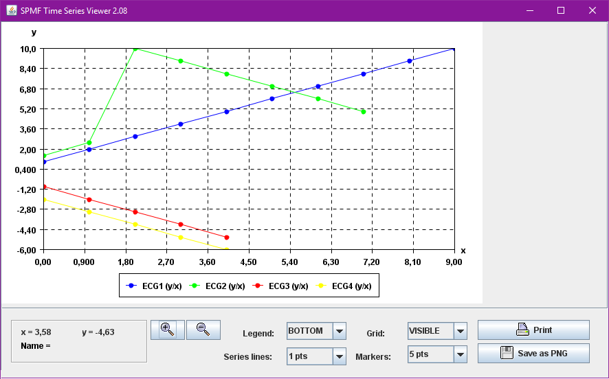
Input file format
The input file format used by the time series viewer defined
as follows. It is a text file. The text file contains one or more time series. Each time series is represented by two lines in the input file. The first line contains the string "@NAME=" followed by the name of the time series. The second line is a list of data points, where data points are floating-point decimal numbers separated by a separator character (here the ',' symbol).
For example, for the previous example, the input file is defined
as follows:
@NAME=ECG1
1,2,3,4,5,6,7,8,9,10
@NAME=ECG2
1.5,2.5,10,9,8,7,6,5
@NAME=ECG3
-1,-2,-3,-4,-5
@NAME=ECG4
-2.0,-3.0,-4.0,-5.0,-6.0
Consider the first two lines. It indicates that the first time series name is "ECG1" and that it consits of the data points: 1, 2, 3, 4, 5, 6, 7, 8, 9, and 10. Then, three other time series are provided in the same file, which follows the same format.
Implementation details
The time series viewer has been implemented by reusing and extending some code provided by Yuriy Guskov under the MIT License for displaying charts.
Example 130 : Calculate moving average of time series
How to run this example?
- If you are using the graphical interface, (1)
choose the "Calculate_moving_average_of_time_series" algorithm, (2) select the input file "contextSAX.txt", (3) set the separator to the comma ',' (4) set the window size to 4, and then (5) click "Run algorithm".
- If you want to execute this example from the command line,
then execute this command:
java -jar spmf.jar run Calculate_moving_average_of_time_series contextSAX.txt output.txt 4 ,
in a folder containing spmf.jar and the example input file contextSAX.txt.
- If you are using the source code version of SPMF, to
run respectively this example, launch
the file "MainTestMovingAverageFromFileToFile.java"in
the package ca.pfv.SPMF.tests.
What is the calculation of the moving average for time series?
Calculating the moving average is a simple but popular way of smoothing a time series to remove noise. It takes as parameter a window size w (a number of data point). Then, for a time series, it replaces each data point by the average of its value plus the values of the (w-1) previous data points.
What is the input of this algorithm?
The input is one or more time series. A time series is a sequence of floating-point decimal numbers (double values). A time-series can also have a name (a string).
Time series are used in many applications. An example of time series is the price of a stock on the stock market over time. Another example is a sequence of temperature readings collected using sensors.
For this example, consider the four following time series:
| Name |
Data points |
| ECG1 |
1,2,3,4,5,6,7,8,9,10 |
| ECG2 |
1.5,2.5,10,9,8,7,6,5 |
| ECG3 |
-1,-2,-3,-4,-5 |
| ECG4 |
-2.0,-3.0,-4.0,-5.0,-6.0 |
This example time series database is provided in the file contextSAX.txt of the SPMF distribution.
In SPMF, to read a time-series file, it is necessary to indicate the "separator", which is the character used to separate data points in the input file. In this example, the "separator" is the comma ',' symbol.
To calculate the moving average, it is also necessary to provide a window size w, which is a number of data points. In this example, this parameter will be set to 4 data points. Thus, the moving average will be calculated for each of the above time series using a window size of 4 data points.
What is the output?
The output is the moving average of the time series received as input. The moving average is calculated by replacing each data point in each time series by the average of its value plus the values of the w-1 previous data points in the same time series.
For example, in the above example, if the window size is set to 4 data points, the result is:
| Name |
Data points |
| ECG1_MAVG |
1.0,1.5,2.0,2.5,3.5,4.5,5.5,6.5,7.5,8.5 |
| ECG2_MAVG |
1.5,2.0,4.666666666666667,5.75,7.375,8.5,7.5,6.5 |
| ECG3_MAVG |
-1.0,-1.5,-2.0,-2.5,-3.5 |
| ECG4_MAVG |
-2.0,-2.5,-3.0,-3.5,-4.5 |
To see the result visually, it is possible to use the SPMF time series viewer, described in another example of this documentation. Here is the result:
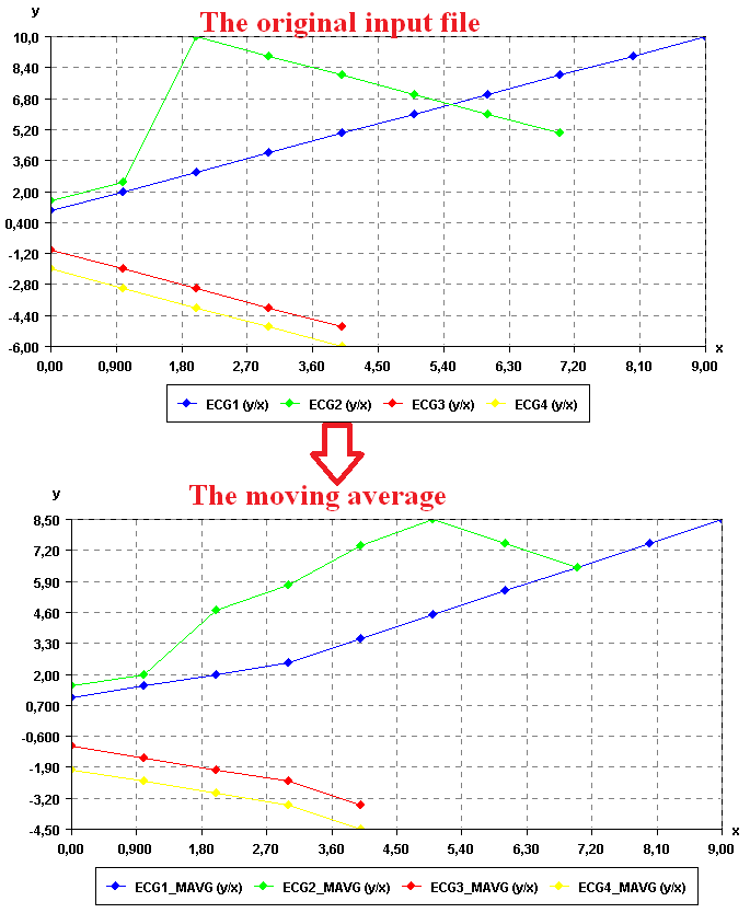
It is possible to see that the time series are less noisy. For example, the time series "ECG3" is much more smooth after applying the moving average.
Input file format
The input file format used by the time series viewer defined
as follows. It is a text file. The text file contains one or more time series. Each time series is represented by two lines in the input file. The first line contains the string "@NAME=" followed by the name of the time series. The second line is a list of data points, where data points are floating-point decimal numbers separated by a separator character (here the ',' symbol).
For example, for the previous example, the input file is defined
as follows:
@NAME=ECG1
1,2,3,4,5,6,7,8,9,10
@NAME=ECG2
1.5,2.5,10,9,8,7,6,5
@NAME=ECG3
-1,-2,-3,-4,-5
@NAME=ECG4
-2.0,-3.0,-4.0,-5.0,-6.0
Consider the first two lines. It indicates that the first time series name is "ECG1" and that it consits of the data points: 1, 2, 3, 4, 5, 6, 7, 8, 9, and 10. Then, three other time series are provided in the same file, which follows the same format.
Output file format
The output file format is the same as the input format.
@NAME=ECG1_MAVG
1.0,1.5,2.0,2.5,3.5,4.5,5.5,6.5,7.5,8.5
@NAME=ECG2_MAVG
1.5,2.0,4.666666666666667,5.75,7.375,8.5,7.5,6.5
@NAME=ECG3_MAVG
-1.0,-1.5,-2.0,-2.5,-3.5
@NAME=ECG4_MAVG
-2.0,-2.5,-3.0,-3.5,-4.5
Implementation details
It is sometimes said that the moving average of a time series should not include the first w-1 points because for these points there is not enough previous points for calculating the average with w points. In this implementation, a design decision is that the moving average should contain as many data points as the original time series. To calculate the moving average of the first w-1 points, it was decided that the first point of the moving average is identical to the first point in the original time series, the second point is the average the two first points, .. the w-1-th point is the average of the w-1 first points of the original time series. This is a design decision.
Where can I get more information about the moving average?
The moving average is a very basic operation for time series. It is described in many websites and books.
Example 131 : Calculate the piecewise aggregate approximation of time series
How to run this example?
- If you are using the graphical interface, (1)
choose the "Visualize_time_series" algorithm, (2) select the input file "contextSAX.txt", (3) set the separator to the comma ',' (4) set the number of segment to 3, and then (5) click "Run algorithm".
- If you want to execute this example from the command line,
then execute this command:
java -jar spmf.jar run Calculate_piecewise_aggregate_approx_of_time_series contextSAX.txt output.txt 3 ,
in a folder containing spmf.jar and the example input file contextSAX.txt.
- If you are using the source code version of SPMF, to
run respectively this example, launch
the file "MainTestPAAFromFileToFile.java"in
the package ca.pfv.SPMF.tests.
What is this algorithm?
Calculating the piecewise aggregate approximation (PAA) of a time series is a popular and simple way of reducing the number of data points in a time series (a way of doing dimensionality reduction).
The idea is very simple. Let's say that a time series contains n data points, and that we want to reduce the time series to w data points, such that w < n. The PAA representation of the time series with w segments is obtained by performing the following process. The time series is divided into w segments and each segment is replaced by the average of its data points.
What is the input of this algorithm?
The input is one or more time series. A time series is a sequence of floating-point decimal numbers (double values). A time-series can also have a name (a string).
Time series are used in many applications. An example of time series is the price of a stock on the stock market over time. Another example is a sequence of temperature readings collected using sensors.
For this example, consider the four following time series:
| Name |
Data points |
| ECG1 |
1,2,3,4,5,6,7,8,9,10 |
| ECG2 |
1.5,2.5,10,9,8,7,6,5 |
| ECG3 |
-1,-2,-3,-4,-5 |
| ECG4 |
-2.0,-3.0,-4.0,-5.0,-6.0 |
This example time series database is provided in the file contextSAX.txt of the SPMF distribution.
In SPMF, to read a time-series file, it is necessary to indicate the "separator", which is the character used to separate data points in the input file. In this example, the "separator" is the comma ',' symbol.
To calculate the piecewise aggregate approximation of a time series, it is necessary to provide a number of segments w, which is the number of data points to be output for each time series. In this example, this parameter will be set to 4 data points. Thus, the piecewise aggregate approximation will be calculated for each of the above time series to produce 4 data points.
What is the output?
The output is the piecewise aggregate approximation of each time series received as input. Let's say that a time series contains n data points, and that we want to reduce the time series to w data points, such that w < n. The PAA representation of the time series with w segments is obtained by performing the following process. The time series is divided into w segments and each segment is replaced by the average of its data points.
For example, in the above example, if the number of segments (data points) is set to 4 data points, the result is:
| Name |
Data points |
| ECG1_PAA |
2.2,5.500000000000001,8.799999999999999 |
| ECG2_PAA |
3.999999999999999,8.500000000000002,5.875 |
| ECG3_PAA |
-1.4000000000000001,-3.0,-4.6 |
| ECG4_PAA |
-2.4,-4.000000000000001,-5.599999999999999 |
To see the result visually, it is possible to use the SPMF time series viewer, described in another example of this documentation. Here is the result:
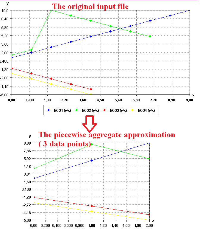
It is possible to see that the number of data points has been reduced while still keeping the shape of the original curve for each time series.
Note that, the implementation of PAA applies PAA independently on each time series. Thus, as seen above, if the time series do not contain the same number of data points, they may not be aligned anymore after applying the PAA transformation. For real applications though, most time series database will contains time series having the same number of data points. So this should not be an issue.
Input file format
The input file format used by this algorithm is efined
as follows. It is a text file. The text file contains one or more time series. Each time series is represented by two lines in the input file. The first line contains the string "@NAME=" followed by the name of the time series. The second line is a list of data points, where data points are floating-point decimal numbers separated by a separator character (here the ',' symbol).
For example, for the previous example, the input file is defined
as follows:
@NAME=ECG1
1,2,3,4,5,6,7,8,9,10
@NAME=ECG2
1.5,2.5,10,9,8,7,6,5
@NAME=ECG3
-1,-2,-3,-4,-5
@NAME=ECG4
-2.0,-3.0,-4.0,-5.0,-6.0
Consider the first two lines. It indicates that the first time series name is "ECG1" and that it consits of the data points: 1, 2, 3, 4, 5, 6, 7, 8, 9, and 10. Then, three other time series are provided in the same file, which follows the same format.
Output file format
The output file format is the same as the input format.
@NAME=ECG1_PAA
2.2,5.500000000000001,8.799999999999999
@NAME=ECG2_PAA
3.999999999999999,8.500000000000002,5.875
@NAME=ECG3_PAA
-1.4000000000000001,-3.0,-4.6
@NAME=ECG4_PAA
-2.4,-4.000000000000001,-5.599999999999999
Where can I get more information about the moving average?
The concept of Piecewise Aggregate Approximation is described in the paper of Lin et al. (2007):
Lin, J., Keogh, E., Wei, L., Lonardi, S.: Experiencing SAX: a novel symbolic representation of time series. Data Mining and Knowledge Discovery 15, 107–144 (2007)
Example 132 : Split time series by length
How to run this example?
- If you are using the graphical interface, (1)
choose the "Split_time_series_by_length" algorithm, (2) select the input file "contextSAX.txt", (3) set the separator to the comma ',' (4) set the size of segment to 3, and then (5) click "Run algorithm".
- If you want to execute this example from the command line,
then execute this command:
java -jar spmf.jar run Split_time_series_by_length contextSAX.txt output.txt 3 ,
in a folder containing spmf.jar and the example input file contextSAX.txt.
- If you are using the source code version of SPMF, to
run respectively this example, launch
the file "MainTestSplitTimeSeriesByLength_FileToFile.java"in
the package ca.pfv.SPMF.tests.
What is this algorithm?
This algorithm takes one or more time series as input. Then it split each time series into several time series. The criteria for spliting the time series is a maximum number of data points per time series (called the "segment size"). For example, if a time series contains 9 data points and the maximum number of data points is set to 3, the time series will be split into three time series of 3 data points each.
This simple algorithm is useful for spliting very long time series into several time series. For example, if one has a temperature reading time series for several years, it would be possible to split the time series by periods of 30 days.
What is the input of this algorithm?
The input is one or more time series. A time series is a sequence of floating-point decimal numbers (double values). A time-series can also have a name (a string).
Time series are used in many applications. An example of time series is the price of a stock on the stock market over time. Another example is a sequence of temperature readings collected using sensors.
For this example, consider the four following time series:
| Name |
Data points |
| ECG1 |
1,2,3,4,5,6,7,8,9,10 |
| ECG2 |
1.5,2.5,10,9,8,7,6,5 |
| ECG3 |
-1,-2,-3,-4,-5 |
| ECG4 |
-2.0,-3.0,-4.0,-5.0,-6.0 |
This example time series database is provided in the file contextSAX.txt of the SPMF distribution.
In SPMF, to read a time-series file, it is necessary to indicate the "separator", which is the character used to separate data points in the input file. In this example, the "separator" is the comma ',' symbol.
To split the data, it is required to provide a maximum number of data points per time series (segment size) for spliting the time series. For example, if a time series contains 9 data points and the maximum number of data points is set to 3, the time series will be split into three time series of 3 data points each.
What is the output?
The output is the set of time series that has been obtained by splitting the time series taken as input.
For example, in the above example, if the number of segments (data points) is set to 3 data points, the result is:
| Name |
Data points |
| ECG1_PART0 |
1.0,2.0,3.0 |
| ECG1_PART1 |
4.0,5.0,6.0 |
| ECG1_PART2 |
7.0,8.0,9.0 |
| ECG1_PART3 |
10.0 |
| ECG2_PART0 |
1.5,2.5,10.0 |
| ECG2_PART1 |
9.0,8.0,7.0 |
| ECG2_PART2 |
6.0,5.0 |
| ECG3_PART0 |
-1.0,-2.0,-3.0 |
| ECG3_PART1 |
-4.0,-5.0 |
| ECG4_PART0 |
-2.0,-3.0,-4.0 |
| ECG4_PART1 |
-5.0,-6.0 |
To see the result visually, it is possible to use the SPMF time series viewer, described in another example of this documentation. Here is the result:
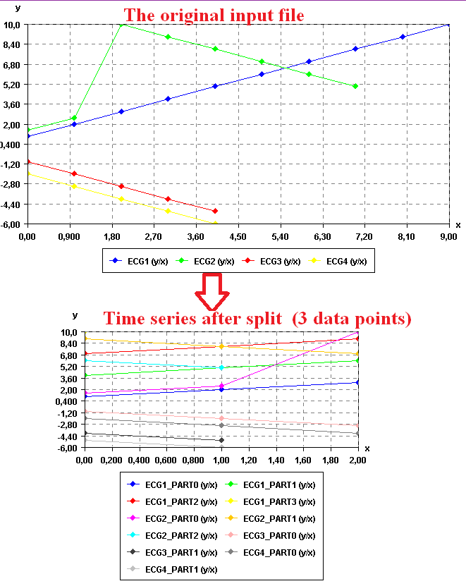
Input file format
The input file format used by this algorithm is efined
as follows. It is a text file. The text file contains one or more time series. Each time series is represented by two lines in the input file. The first line contains the string "@NAME=" followed by the name of the time series. The second line is a list of data points, where data points are floating-point decimal numbers separated by a separator character (here the ',' symbol).
For example, for the previous example, the input file is defined
as follows:
@NAME=ECG1
1,2,3,4,5,6,7,8,9,10
@NAME=ECG2
1.5,2.5,10,9,8,7,6,5
@NAME=ECG3
-1,-2,-3,-4,-5
@NAME=ECG4
-2.0,-3.0,-4.0,-5.0,-6.0
Consider the first two lines. It indicates that the first time series name is "ECG1" and that it consits of the data points: 1, 2, 3, 4, 5, 6, 7, 8, 9, and 10. Then, three other time series are provided in the same file, which follows the same format.
Output file format
The output file format is the same as the input format.
@NAME=ECG1_PART0
1.0,2.0,3.0
@NAME=ECG1_PART1
4.0,5.0,6.0
@NAME=ECG1_PART2
7.0,8.0,9.0
@NAME=ECG1_PART3
10.0
@NAME=ECG2_PART0
1.5,2.5,10.0
@NAME=ECG2_PART1
9.0,8.0,7.0
@NAME=ECG2_PART2
6.0,5.0
@NAME=ECG3_PART0
-1.0,-2.0,-3.0
@NAME=ECG3_PART1
-4.0,-5.0
@NAME=ECG4_PART0
-2.0,-3.0,-4.0
@NAME=ECG4_PART1
-5.0,-6.0
Example 133 : Split time series by number of segments
How to run this example?
- If you are using the graphical interface, (1)
choose the "Split_time_series_by_number_of_segments" algorithm, (2) select the input file "contextSAX.txt", (3) set the separator to the comma ',' (4) set the number of segment to 2, and then (5) click "Run algorithm".
- If you want to execute this example from the command line,
then execute this command:
java -jar spmf.jar run Split_time_series_by_number_of_segments contextSAX.txt output.txt 2 ,
in a folder containing spmf.jar and the example input file contextSAX.txt.
- If you are using the source code version of SPMF, to
run respectively this example, launch
the file "MainTestSplitTimeSeriesByNumberOfSegments_FileToFile.java"in
the package ca.pfv.SPMF.tests.
What is this algorithm?
This algorithm takes one or more time series as input. Then it split each time series into several time series. The criteria for spliting the time series is a given number of segments specified by the user. If the user specify w segments, then each time series will be split into w time series. This simple algorithm is useful for spliting very long time series into several time series.
What is the input of this algorithm?
The input is one or more time series. A time series is a sequence of floating-point decimal numbers (double values). A time-series can also have a name (a string).
Time series are used in many applications. An example of time series is the price of a stock on the stock market over time. Another example is a sequence of temperature readings collected using sensors.
For this example, consider the four following time series:
| Name |
Data points |
| ECG1 |
1,2,3,4,5,6,7,8,9,10 |
| ECG2 |
1.5,2.5,10,9,8,7,6,5 |
| ECG3 |
-1,-2,-3,-4,-5 |
| ECG4 |
-2.0,-3.0,-4.0,-5.0,-6.0 |
This example time series database is provided in the file contextSAX.txt of the SPMF distribution.
In SPMF, to read a time-series file, it is necessary to indicate the "separator", which is the character used to separate data points in the input file. In this example, the "separator" is the comma ',' symbol.
To split the data, it is required to provide a number of segments w per time series for spliting the time series.
What is the output?
The output is the set of time series that has been obtained by splitting each time series into w time series.
For example, in the above example, if the number of segments (data points) is set to 3 data points, the result is:
| Name |
Data points |
| ECG1_PART0 |
1.0,2.0,3.0,4.0,5.0 |
| ECG1_PART1 |
6.0,7.0,8.0,9.0,10.0 |
| ECG2_PART0 |
1.5,2.5,10.0,9.0 |
| ECG2_PART1 |
8.0,7.0,6.0,5.0 |
| ECG3_PART0 |
-1.0,-2.0,-3.0 |
| ECG3_PART1 |
-4.0,-5.0 |
| ECG4_PART0 |
-2.0,-3.0,-4.0 |
| ECG4_PART1 |
-5.0,-6.0 |
To see the result visually, it is possible to use the SPMF time series viewer, described in another example of this documentation. Here is the result:
Input file format
The input file format used by this algorithm is efined
as follows. It is a text file. The text file contains one or more time series. Each time series is represented by two lines in the input file. The first line contains the string "@NAME=" followed by the name of the time series. The second line is a list of data points, where data points are floating-point decimal numbers separated by a separator character (here the ',' symbol).
For example, for the previous example, the input file is defined
as follows:
@NAME=ECG1
1,2,3,4,5,6,7,8,9,10
@NAME=ECG2
1.5,2.5,10,9,8,7,6,5
@NAME=ECG3
-1,-2,-3,-4,-5
@NAME=ECG4
-2.0,-3.0,-4.0,-5.0,-6.0
Consider the first two lines. It indicates that the first time series name is "ECG1" and that it consits of the data points: 1, 2, 3, 4, 5, 6, 7, 8, 9, and 10. Then, three other time series are provided in the same file, which follows the same format.
Output file format
The output file format is the same as the input format.
@NAME=ECG1_PART0
1.0,2.0,3.0,4.0,5.0
@NAME=ECG1_PART1
6.0,7.0,8.0,9.0,10.0
@NAME=ECG2_PART0
1.5,2.5,10.0,9.0
@NAME=ECG2_PART1
8.0,7.0,6.0,5.0
@NAME=ECG3_PART0
-1.0,-2.0,-3.0
@NAME=ECG3_PART1
-4.0,-5.0
@NAME=ECG4_PART0
-2.0,-3.0,-4.0
@NAME=ECG4_PART1
-5.0,-6.0
Example 134 : Convert time series to sequences using the SAX algorithm
How to run this example?
- If you are using the graphical interface, (1)
choose the "Convert_time_series_to_sequence_database_using_SAX" algorithm, (2) select the input file "contextSAX.txt", (3) set the separator to the comma ',' (4) set the number of segment to 3, (5) set the number of symbols to 4, and then (6) click "Run algorithm".
- If you want to execute this example from the command line,
then execute this command:
java -jar spmf.jar run Convert_time_series_to_sequence_database_using_SAX contextSAX.txt output.txt 3 4 ,
in a folder containing spmf.jar and the example input file contextSAX.txt.
- If you are using the source code version of SPMF, to
run respectively this example, launch
the file "MainTestConvertTimeSeriesFiletoSequenceFileWithSAX.java"in
the package ca.pfv.SPMF.tests.
What is this algorithm?
Calculating the SAX of a time series is a popular and simple way of transforming time series to a symbolic representation. In other words, SAX is a way of transforming a time series (a sequence of numbers) to a sequence of symbols.
This implementation takes a set of one or more time series as input. Then, it transform the time series to their SAX representation.
The SAX algorithm was proposed by Lin et al. (2007) and is quite popular.
The interest of applying the SAX algorithm to time series, is that after obtaining the SAX representation, we can apply traditional symbolic pattern mining algorithms such as sequential pattern mining and sequential rule mining algorithms, also offered in SPMF.
What is the input of this algorithm?
The input is one or more time series. A time series is a sequence of floating-point decimal numbers (double values). A time-series can also have a name (a string).
Time series are used in many applications. An example of time series is the price of a stock on the stock market over time. Another example is a sequence of temperature readings collected using sensors.
For this example, consider the four following time series:
| Name |
Data points |
| ECG1 |
1,2,3,4,5,6,7,8,9,10 |
| ECG2 |
1.5,2.5,10,9,8,7,6,5 |
| ECG3 |
-1,-2,-3,-4,-5 |
| ECG4 |
-2.0,-3.0,-4.0,-5.0,-6.0 |
This example time series database is provided in the file contextSAX.txt of the SPMF distribution.
In SPMF, to read a time-series file, it is necessary to indicate the "separator", which is the character used to separate data points in the input file. In this example, the "separator" is the comma ',' symbol.
To calculate the SAX representation of a time series, it is necessary to also provides two additional parameters: a number of segments w, and a number of symbols v.
What is the output?
The output is the SAX representation of each time series received as input. For a given time series, the SAX representation is calculated as follows. First, the time series is divided into w segments, and each segments is replaced by the average of its data points. This is called the piecewise approximate aggregation (PAA) of the time series. Then, the value of each segment is replaced by a symbol. The number of symbol and the number of segment is selected by the user.
Now, the main question is how the symbols are chosen? The main idea in SAX is to assume that values follow a normal distribution and to choose the symbol to represent various interval of values such that each interval is equally probable under the normal distribution (see the paper of Lin et al. 2007 for a more detailed explanation).
For example, in the above example, if the number of segments (data points) is set to 3 data points, and the number of symbols is set to 4, the sax algorithm will create four symbols:
| Symbol |
Interval of values represented by this symbol |
| a |
[-Infinity,-0.9413981789451658] |
| b |
[-0.9413981789451658,2.4642857142857144] |
| c |
[2.4642857142857144,5.869969607516595] |
| d |
[5.869969607516595,Infinity] |
Using the above symbols, the SAX algorithm generate the following SAX representation of each time series:
| Name |
Data points |
| ECG1_PAA |
b, c, d, |
| ECG2_PAA |
c, d, d |
| ECG3_PAA |
a, a, a |
| ECG4_PAA |
a, a, a |
After obtaining this representation, it is possible to apply traditional pattern mining algorithm on the sequences of symbols. For example, in SPMF, several algorithms are provided for sequential pattern mining and sequential rule mining, which can be applied on sequence of symbols.
Input file format
The input file format used by this algorithm is efined
as follows. It is a text file. The text file contains one or more time series. Each time series is represented by two lines in the input file. The first line contains the string "@NAME=" followed by the name of the time series. The second line is a list of data points, where data points are floating-point decimal numbers separated by a separator character (here the ',' symbol).
For example, for the previous example, the input file is defined
as follows:
@NAME=ECG1
1,2,3,4,5,6,7,8,9,10
@NAME=ECG2
1.5,2.5,10,9,8,7,6,5
@NAME=ECG3
-1,-2,-3,-4,-5
@NAME=ECG4
-2.0,-3.0,-4.0,-5.0,-6.0
Consider the first two lines. It indicates that the first time series name is "ECG1" and that it consits of the data points: 1, 2, 3, 4, 5, 6, 7, 8, 9, and 10. Then, three other time series are provided in the same file, which follows the same format.
Output file format
The output file format is a sequence database containing one or more sequence. It is defined as follows. The first line contains the string "@CONVERTED_FROM_TIME_SERIES" to indicate that this file was obtained by converting some time series to sequences. The following defines the symbols produced by the SAX algorithm. Each line defining a symbol starts with "@ITEM=" and is followed by a symbol name (a positive integer), followed by "=", followed by the interval of values represented by this symbol. Then, the following lines are the sequences of symbols. Each sequence is represented by two lines. The first line contains "@NAME=" and is followed by the name of the sequence. The second line is the sequence. A sequence is a list of symbols separated by -1, and ending with a -2.
For example, the output of this example is:
@CONVERTED_FROM_TIME_SERIES
@ITEM=1=[-Infinity,-0.9413981789451658]
@ITEM=2=[-0.9413981789451658,2.4642857142857144]
@ITEM=3=[2.4642857142857144,5.869969607516595]
@ITEM=4=[5.869969607516595,Infinity]
@NAME=ECG1
2 -1 3 -1 4 -1 -2
@NAME=ECG2
3 -1 4 -1 4 -1 -2
@NAME=ECG3
1 -1 1 -1 1 -1 -2
@NAME=ECG4
1 -1 1 -1 1 -1 -2
The first five lines indicates that four symbols are defined called 1, 2, 3, 4, which were called a, b, c, d previously in this example.
Then, four sequences are defined.
The first sequence is 2, 3, 4, which was previously called b, c, d in this example.
Optional parameter
This implementation of SAX offers an optional parameter called "deactivatePAA". It is this used to directly convert timeseries to their SAX representation without first performing the transformation to the PAA representation. This parameter is optional. It is useful when converting several time series of different lengths to their SAX representation. When this parameter is set to true, the algorithm will preserve the original lengths of the time series rather than converting all of them to the same length. To this use this parameter in the user interface of SPMF, type the value "true". For the command line of SPMF, add the value "true" at the end of the line. For example: java -jar spmf.jar run Convert_time_series_to_sequence_database_using_SAX contextSAX.txt output.txt 3 4 , true
Where can I get more information about the moving average?
The SAX representation is described in the paper of Lin et al. (2007):
Lin, J., Keogh, E., Wei, L., Lonardi, S.: Experiencing SAX: a novel symbolic representation of time series. Data Mining and Knowledge Discovery 15, 107–144 (2007)
Example 135 : Clustering Texts with a text clusterer
How to run this example?
- If you are using the graphical interface, (1)
choose the "TextClusterer"
algorithm, (2) select the input file "input_text_clustering.txt",
(3) set the output file name (e.g. "output.txt")
(4) set "Perform stemming:"
to true, (5) set "Remove stopwords:"
to true, and (5) click "Run algorithm".
- If you want to execute this example from the command line,
then execute this command:
java -jar spmf.jar run TextClusterer input_text_clustering.txt
output.txt true true in a folder containing spmf.jar
and the example input file input_text_clustering.txt.
- If you are using the source code version of SPMF, launch
the file "MainTestTextClusterer.java"
in the package ca.pfv.SPMF.tests.
What is this algorithm?
The algorithm is a text clusterer implemented
by Sabarish Raghu. It can group texts automatically
into clusters. Furthermore, it offers the possiblity of performing
stemming and removing stop words before performing clustering.
The text clusterer works as follows:
1. Load the input file
2. Remove the stopwords (optional)
3. Stem the words (optional)
4. Calculate tf*idf value for each record in the
input file.
5. Calculate similarity matrix by using the tfidf values of the records.
6. Take most similar records per each record and make them as clusters
initially.
7. Use the transitive rule A,B are most similar and B,C are most
similar; A and C are likely to be similar. This imply that A, B, C are
in the same cluster.
8. Merge the clusters based on the above rule for all the records.
9. Write the final output i.e,; final sets of clusters to the output
file.
StopWords
Words that are insignificant to identify the clusters. This algorithm
by defauly uses the list of most popular stopwords. Anyways we can
define our own stopword list or even not remove any word.
Stemming
Stemming is deriving the base word of a word.
For example: Identification is stemmed to Identity
For stemming, we use the famous Porter stemmer algorithm, which
uses rules given by Porter to stem the words. This implementation is
taken from Brian Goetz's implementation from the internet.
tf:term frequency
Term frequency defines how frequently a term occur in a document
Idf:Inverse document frequency
Inverse document frequency is the frequency of a word in the whole set
of documents.
similarity matrix:
2 dimensional matrix representation of a record's similarity with all
other records.
What is the input?
The input is a text file.
Each line of the text file represents a text.
A line starts with an integer id. Then, it is followed by a tab,
and then a text where words are separated by spaces.
An example of input is provided in the file "input_text_clustering.txt"
of the SPMF distribution. It contains 100 texts (100 lines). For
example, here are two lines from this file:
692770 inventory taker description team members required
physically count inventory various retailers enter information
equipment inventory counted varies depending type store audited items
may located floor tables shelves various heights items generally
counted shelves may moved required inventories take approximately hours
complete however may take longer depending size store level inventory
counted
574319 leading hotel furniture supplier seeking project managers
manage national international accounts bid packages unique exciting
opportunity right individuals qualified applicants should send resumes
talli globalallies com phone calls please
What is the output?
The output is a set of clusters of similar texts.
The output file format is defined as follows.
The first line indicates the file format. Then, each following line
contains a text id followed by a cluster id. For example, here are the
first five lines of the output file obtained by applying the text
clusterer on the sample input file:
RecordId Clusternum
171056 0
770853 0
247263 1
870007 1
Results can be interpreted as follows. The texts with ids "171056"
and "770853" both belongs to the same cluster, having the id "0".
Moreover, the texts with ids "247263" and "870007" both belongs to the
same cluster, having the id "1".
Example 136 : Creating a decision tree with the ID3
algorithm to predict the value of a target attribute
How to run this example?
To run this example with the source code version of SPMF,
launch the file "MainTestID3.java"
in the package ca.pfv.SPMF.tests.
This example is not available in the release version of
SPMF.
What is the ID3 algorithm?
The ID3 algorithm is a classic data mining
algorithm for classifying instances (a classifier). It is
well-known and described in many artificial intelligence and data
mining books.
What is the input?
The input is a set of training data for building a decision tree.
For instance, in this example, we use the following database (from
the book "Machine Learning by Tom Mitchell). This database is provided
in the file "tennis.txt" of the SPMF distribution.
This database defines five attributes and contains fourteen
instances.
| outlook |
temp |
humid |
wind |
play? |
| sunny |
hot |
high |
weak |
no |
| sunny |
hot |
high |
strong |
no |
| overcast |
hot |
high |
weak |
yes |
| rain |
mild |
high |
weak |
yes |
| rain |
cool |
normal |
weak |
yes |
| rain |
cool |
normal |
strong |
no |
| overcast |
cool |
normal |
strong |
yes |
| sunny |
mild |
high |
weak |
no |
| sunny |
cool |
normal |
weak |
yes |
| rain |
mild |
normal |
weak |
yes |
| sunny |
mild |
normal |
strong |
yes |
| overcast |
mild |
high |
strong |
yes |
| overcast |
hot |
normal |
weak |
yes |
| rain |
mild |
high |
strong |
no |
What is the output?
By applying the ID3 algorithm, a decision tree
is created. To create the decision tree, we have to choose a target
attribute. Here, we choose the attribute "play".
The following decision tree is created:
We can now use the tree to predict the value of the target
attribute "play" for a new instance.
For example, consider this new instance, where the value for
"play" is unknown.
By applying the decision tree, the value for the attribute "play"
for this instance is "yes".
Input file format
The input file format is a text file. The first lines contains a
list of attribute names separated by a single space. A attribute name
is simply a string without spaces. The next lines represents instances,
where each line contains a string value for each attribute, separated
by single spaces. For example, consider the file "tennis.txt" of the
previous example.
play outlook temp humid wind
no sunny hot high weak
no sunny hot high strong
yes overcast hot high weak
yes rain mild high weak
yes rain cool normal weak
no rain cool normal strong
yes overcast mild high strong
no sunny mild high weak
yes sunny cool normal weak
yes rain mild normal weak
yes sunny mild normal strong
yes overcast hot normal weak
yes overcast cool normal strong
no rain mild high strong
The first line defines the attribute names : "play", "outlook",
"temp", "humid" and "wind". Then, consider the second line. It
represents an instance having the value "no", "sunny", "hot", "high"
and "weak" respectively for the five attributes. The next lines follow
the same format.
Output file format
There is no output file for the ID3 algorithm. It is only
available in the source code version of SPMF and it does not generate
an output file.
Where can I get more information about the ID3 algorithm?
The ID3 algorithm was proposed by Quinlan (1986). It is one of the
most popular algorithm for learning decision trees. By searching on the
web, you can find plenty of information on this algorithm. It is also
described in several data mining books and artificial intelligence
books.
Example 137 : Converting a Sequence Database to SPMF
Format
How to run this example?
- If you are using the graphical interface, (1)
choose the "Convert_a_sequence_database_to_SPMF_format"
algorithm, (2) select the input file "contextCSV.txt",
(3) set the output file name (e.g. "output.txt")
(4) set input_format = CSV_INTEGER
and sequence count = 5.(5) click
"Run algorithm".
- If you want to execute this example from the command line,
then execute this command:
java -jar spmf.jar run Convert_a_sequence_database_to_SPMF_format
contextCSV.txt output.txt CSV 5 in a folder containing spmf.jar and the example input file contextCSV.txt.
- If you are using the source code version of SPMF, launch
the file "MainTestConvertSequenceDatabase.java"
in the package ca.pfv.SPMF.tests.
The tool for converting a sequence databases to SPMF format
takes three prameters as input:
- a sequence database,
- the name of the sequence database format (CSV_INTEGER, Kosarak,
Snake, IBMGenerator or BMS),
- the number of sequences to be converted
The algorithm outputs a sequence database in SPMF format.
The CSV_INTEGER format is defined as follows:
- each line is a sequence
- each sequence is a list of items represented by positive integers
(>0) separated by commas.
For example, the follwing sequence databasee is in CSV_INTEGER
format and contains four sequences:
1,2,3,4
5,6,7,8
5,6,7
1,2,3
The Kosarak format is defined as follows:
- each line is a sequence
- each sequence is a list of items represented by integers and
separated by a space.
For example, the follwing sequence databasee is in Kosarak format
and contains four sequences:
1 2 3 4
5 6 7 8
5 6 7
1 2 3
The IBMGenerator format is the format used by the
IBM Data Quest Generator. The format is defined as
follows:
- the file is a binary file in little indian format
- the file is a list of integers without spaces
- a positive integer represents an item
- -1 represents the end of an itemset
- -2 represents the end of a sequence
For example, the follwing sequence databasee is in Kosarak format
and contains four sequences:
1 -1 2 -1 3 -1 4 -1 -2
5 -1 6 -1 7 -1 8 -1 -2
5 -1 6 -1 7 -1 -2
1 -1 2 -1 3 -1 -2
The Snake format is defined as follows:
- each line is a sequence
- each sequence is a list of letters
For example, the follwing sequence databasee is in Snake format and
contains four sequences:
ABCD
ABAB
CACD
ADAC
The BMS format is defined as follows:
- each line contains a sequence id and an item, both represented as
integers
For example, the follwing sequence databasee is in BMS format and
contains four sequences with the ids 10, 20, 30 and 40, respectively:
10 1
10 2
10 3
10 4
20 5
20 6
20 7
20 8
30 5
30 6
30 7
40 1
40 2
40 3
Example 138 : Converting a Transaction Database to SPMF
Format
How to run this example?
- If you are using the graphical interface, (1)
choose the "Convert_a_transaction_database_to_SPMF_format"
algorithm, (2) select the input file "contextCSV.txt",
(3) set the output file name (e.g. "output.txt")
(4) set input_format = CSV_INTEGER
and sequence count = 5.(5) click
"Run algorithm".
- If you want to execute this example from the command line,
then execute this command:
java -jar spmf.jar run Convert_a_transaction_database_to_SPMF_format
contextCSV.txt output.txt CSV_INTEGER 5 in a folder
containing spmf.jar and the example input
file contextCSV.txt.
- If you are using the source code version of SPMF, launch
the file "MainTestConvertTransactionDatabaseCSVtoSPMF.java"
in the package ca.pfv.SPMF.tests.
The tool for converting a transaction databases to SPMF
format. It takes three prameters as input:
- an input file,
- the input file format database format (CSV_INTEGER),
- the number of transactions to be converted
The algorithm outputs a transaction database in SPMF format.
The CSV_INTEGER format is defined as follows:
- each line is a transaction
- each transaction is a list of items represented by positive
integers (>0) separated by commas.
For example, the follwing sequence database is in CSV_INTEGER format
and contains four sequences:
1,2,3,4
5,6,7,8
5,6,7
1,2,3
Other formats will be added eventually.
Example 139 : Converting a Sequence
Database to a Transaction Database
How to run this example?
- If you are using the graphical interface, (1)
choose the "Convert_sequence_database_to_transaction_database"
algorithm, (2) select the input file "contextPrefixspan.txt",
(3) set the output file name (e.g. "output.txt")
and sequence count = 5 (5) click
"Run algorithm".
- If you want to execute this example from the command line,
then execute this command:
java -jar spmf.jar run Convert_sequence_database_to_transaction_database contextPrefixspan.txt
output.txt 5 in a folder containing spmf.jar
and the example input file contextPrefixspan.txt.
- If you are using the source code version of SPMF, launch
the file "MainTestConvertSeqDBToTransDB.java"
in the package ca.pfv.SPMF.tests
What is this tool?
This tool converts a sequence database to a transaction database
by removing the ordering between items. This tool is useful if you have
a sequence database and you want to apply an algorithm that is designed
to be applied on a sequence database. For example, you could take a
sequence database and convert it to a transaction database to then
apply and association rule mining algorithm.
What is the input?
The tool takes two prameters as input:
- an input file (the sequence database),
- the number of lines of the input file to be converted
A sequence database is a set of sequences where
each sequence is a list of itemsets. An itemset is an unordered set of
items. For example, the table shown below contains four sequences. The
first sequence, named S1, contains 5 itemsets. It means that item 1 was
followed by items 1 2 and 3 at the same time, which were followed by 1
and 3, followed by 4, and followed by 3 and 6. It is assumed that items
in an itemset are sorted in lexicographical order. This database is
provided in the file "contextPrefixspan.txt"
of the SPMF distribution. Note that it is assumed that
no items appear twice in the same itemset and that items in an itemset
are lexically ordered.
| ID |
Sequences |
| S1 |
(1), (1 2 3), (1 3), (4), (3 6) |
| S2 |
(1 4), (3), (2 3), (1 5) |
| S3 |
(5 6), (1 2), (4 6), (3), (2) |
| S4 |
(5), (7), (1 6), (3), (2), (3) |
What is the output?
The output is a transaction database in SPMF format. A transaction
database is a set of transactions. Each transaction an unordered set of
items (symbols) represented by positive integers. For example, consider
the following database. The output for this example would be the
following transaction database. It contains five
transactions. The first transaction contains the set of items {1, 3, 4,
6}.
| Transaction id |
Items |
| t1 |
{1, 2, 3, 4, 6} |
| t2 |
{1, 2, 3, 4, 5} |
| t3 |
{1, 2, 3, 4, 5, 6} |
| t4 |
{1, 2, 3, 5, 6, 7} |
Input file format
The input file format is defined as follows. It
is a text file where each line represents a sequence from a sequence
database. Each item from a sequence is a positive integer and items
from the same itemset within a sequence are separated by single space.
Note that it is assumed that items within a same itemset are sorted
according to a total order and that no item can appear twice in the
same itemset. The value "-1" indicates the end of an itemset. The value
"-2" indicates the end of a sequence (it appears at the end of each
line). For example, the input file "contextPrefixSpan.txt" contains the
following four lines (four sequences).
1 -1 1 2 3 -1 1 3 -1 4 -1 3 6 -1 -2
1 4 -1 3 -1 2 3 -1 1 5 -1 -2
5 6 -1 1 2 -1 4 6 -1 3 -1 2 -1 -2
5 -1 7 -1 1 6 -1 3 -1 2 -1 3 -1 -2
The first line represents a sequence where the itemset {1} is
followed by the itemset {1, 2, 3}, followed by the itemset {1, 3},
followed by the itemset {4}, followed by the itemset {3, 6}. The next
lines follow the same format.
Output file format
The output file format is defined as follows.
It is a text file. An item is represented by a positive integer. A
transaction is a line in the text file. In each line (transaction),
items are separated by a single space. It is assumed that all items
within a same transaction (line) are sorted according to a total order
(e.g. ascending order) and that no item can appear twice within the
same line.
For example, for the previous example, the output file is defined
as follows:
1 2 3 4 6
1 2 3 4 5
1 2 3 4 5 6
1 2 3 5 6 7
Example 140 : Converting a
Transaction Database to a Sequence Database
How to run this example?
- If you are using the graphical interface, (1)
choose the "Convert_transaction_database_to_sequence_database"
algorithm, (2) select the input file "contextPasquier99.txt",
(3) set the output file name (e.g. "output.txt")
and sequence count = 5 (5) click
"Run algorithm".
- If you want to execute this example from the command line,
then execute this command:
java -jar spmf.jar run Convert_transaction_database_to_sequence_database
contextPasquier99.txt output.txt 5 in a folder
containing spmf.jar and the example input
file contextPasquier99.txt.
- If you are using the source code version of SPMF, launch
the file "MainTestConvertTransDBtoSeqDB.java"
in the package ca.pfv.SPMF.tests
What is this tool?
This tool converts a transaction database to a sequence database.
It should be used carefully since it assumes that each transaction is a
sequence, and that items in each transaction are sequentially ordered,
which is usually not the case in real-life transaction databases.
What is the input?
The tool takes two prameters as input:
- an input file (the transaction database),
- the number of lines of the input file to be converted
A transaction database is a set of transactions.
Each transaction is a set of items. For example,
consider the following transaction database. It contains 5 transactions
(t1, t2, ..., t5) and 5 items (1,2, 3, 4, 5). For example, the first
transaction represents the set of items 1, 3 and 4. This database is
provided as the file contextPasquier99.txt in the
SPMF distribution. It is important to note that an item is not allowed
to appear twice in the same transaction and that items are assumed to
be sorted by lexicographical order in a transaction.
| Transaction id |
Items |
| t1 |
{1, 3, 4} |
| t2 |
{2, 3, 5} |
| t3 |
{1, 2, 3, 5} |
| t4 |
{2, 5} |
| t5 |
{1, 2, 3, 5} |
What is the output?
The output is a sequence database in SPMF format. A sequence
database is a set of sequences. Each sequence is an ordered list of
itemsets. Each itemset is an unordered set of items (symbols)
represented by positive integers. The output for this example is the
following sequence database. It contains five
sequences. The first sequence indicates that item 1 is followed by item
3, which is followed by item 4.
| Sequence id |
Itemsets |
| s1 |
{1},{3}, {4} |
| s2 |
{2},{3},{5} |
| s3 |
{1}, {2}, {3}, {5} |
| s4 |
{2}, {5}, |
| s5 |
{1}, {2}, {3}, {5} |
Input file format
The input file format is defined as follows. It
is a text file. An item is represented by a positive integer. A
transaction is a line in the text file. In each line (transaction),
items are separated by a single space. It is assumed that all items
within a same transaction (line) are sorted according to a total order
(e.g. ascending order) and that no item can appear twice within the
same line.
For example, for the previous example, the input file is defined
as follows:
1 3 4
2 3 5
1 2 3 5
2 5
1 2 3 5
Output file format
The output file format is defined as follows. It
is a text file where each line represents a sequence from a sequence
database. Each item from a sequence is a positive integer and items
from the same itemset within a sequence are separated by single space.
Note that it is assumed that items within a same itemset are sorted
according to a total order and that no item can appear twice in the
same itemset. The value "-1" indicates the end of an itemset. The value
"-2" indicates the end of a sequence (it appears at the end of each
line). For example, the output file for this example contains five
lines (five sequences).
1 -1 3 -1 4 -1 -2
2 -1 3 -1 5 -1 -2
1 -1 2 -1 3 -1 5 -1 -2
2 -1 5 -1 -2
1 -1 2 -1 3 -1 5 -1 -2
The first line represents a sequence where the item 1 is followed
by item 3, which is followed by item 4.
Example 141 : Generating a Synthetic Sequence Database
How to run this example?
- If you are using the graphical interface, (1)
choose the "Generate_a_sequence_database"
algorithm, (2) set the output file name
(e.g. "output.txt") (3)
choose 100 sequences, 1000 maximum distinct items, 3 items by itemset,
7 itemsets per sequence (4) click "Run algorithm".
- If you want to execute this example from the command line,
then execute this command:
java -jar spmf.jar run Generate_a_sequence_database
no_input_file output.txt 100 1000 3 7 in a folder containing spmf.jar.
- If you are using the source code version of SPMF, launch
the file "MainTestGenerateSequenceDatabase.java"
in the package ca.pfv.SPMF.tests.
What is this tool?
This tool is a random generator of sequence databases. It can be
used to generate synthetic sequence databases to
compare the performance of data mining algorithms that takes a sequence
database as input.
Synthetic databases are often used in the data mining litterature
to evaluate algorithms. In particular, they are useful for comparing
the scalability of algorithms. For example, one can generate sequence
databases having various size and see how the algorithms react in terms
of execution time and memory usage with respect to the database size.
What is the input?
The tool for generating a sequence databases takes
four prameters as input:
1) the number of sequences to be generated (an integer >= 1)
2) the maximum number of distinct item that the database should
contain (an integer >= 1),
3) the number of items that each itemset should contain (an
integer >= 1)
4) the number of itemsets that each sequence should contain (an
integer >= 1)
What is the output?
The algorithm outputs a sequence database respecting these
parameters. The database is generated by using a random number
generator.
Example 142 : Generating a Synthetic Sequence Database
with Timestamps
How to run this example?
- If you are using the graphical interface, (1)
choose the "Generate_a_sequence_database_with_timetamps"
algorithm, (2) set the output file name (e.g. "output.txt") (3) choose 100
sequences, 1000 maximum distinct items, 3 item by itemset, 7 itemsets
per sequence (4) click "Run algorithm".
- If you want to execute this example from the command line,
then execute this command:
java -jar spmf.jar run Generate_a_sequence_database_with_timestamps
no_input_file output.txt 100 1000 3 7 in a folder containing spmf.jar.
- If you are using the source code version of SPMF, launch
the file "MainTestGenerateSequenceDatabaseWithTimeStamps.java"
in the package ca.pfv.SPMF.tests.
What is this tool?
This tool is a random generator of sequence databases
with timestamps. It can be used to generate synthetic
sequence databases with timestamps to compare the performance
of data mining algorithms that takes a sequence database with
timestamps as input.
Synthetic databases are often used in the data mining litterature
to evaluate algorithms. In particular, they are useful for comparing
the scalability of algorithms. For example, one can generate sequence
databases having various size and see how the algorithms react in terms
of execution time and memory usage with respect to the database size.
What is the input?
The tool for generating a sequence databases with
timestamps takes four prameters as input:
1) the number of sequences to be generated (an integer >= 1)
2) the maximum number of distinct item that the database should
contain (an integer >= 1),
3) the number of items that each itemset should contain (an
integer >= 1)
4) the number of itemsets that each sequence should contain (an
integer >= 1)
What is the output?
The algorithm outputs a sequence database with timestamps
respecting these parameters. The database is generated by using a
random number generator.
Example 143 : Generating a Synthetic Transaction Database
How to run this example?
- If you are using the graphical interface, (1)
choose the "Generate_a_transaction_database"
algorithm, (2) set the output file name (e.g. "output.txt") (3) choose 100
transactions, 1000 maximum distinct items and 10 items per transaction
(4) click "Run algorithm".
- If you want to execute this example from the command line,
then execute this command:
java -jar spmf.jar run Generate_a_transaction_database
no_input_file output.txt 100 1000 10 in a folder containing spmf.jar.
- If you are using the source code version of SPMF, launch
the file "MainTestGenerateTransactionDatabase.java"
in the package ca.pfv.SPMF.tests.
What is this tool?
This tool is a random generator of transaction databases.
It can be used to generate synthetic transaction databases
with timestamps to compare the performance of data mining
algorithms that takes a transaction database as input.
Synthetic databases are often used in the data mining litterature
to evaluate algorithms. In particular, they are useful for comparing
the scalability of algorithms. For example, one can generate sequence
databases having various size and see how the algorithms react in terms
of execution time and memory usage with respect to the database size.
What is the input?
The tool for generating a transaction takes
three prameters as input:
1) the number of transactions to be generated (an integer
>= 1)
2) the maximum number of distinct item that the database
should contain (an integer >= 1),
3) the number of items that each transaction should contain
(an integer >= 1)
What is the output?
The algorithm outputs a transaction database database respecting
the parameters provided. A random number generator is used to generate
the database.
A transaction database is a set of transactions.
Each transaction is a set of items. For example,
consider the following transaction database. It contains 5 transactions
(t1, t2, ..., t5) and 5 items (1,2, 3, 4, 5). For example, the first
transaction represents the set of items 1, 3 and 4. It is important to
note that an item is not allowed to appear twice in the same
transaction and that items are assumed to be sorted by lexicographical
order in a transaction.
| Transaction id |
Items |
| t1 |
{1, 3, 4} |
| t2 |
{2, 3, 5} |
| t3 |
{1, 2, 3, 5} |
| t4 |
{2, 5} |
| t5 |
{1, 2, 3, 5} |
Output file format
The output file format is defined as follows.
It is a text file. An item is represented by a positive integer. A
transaction is a line in the text file. In each line (transaction),
items are separated by a single space. It is assumed that all items
within a same transaction (line) are sorted according to a total order
(e.g. ascending order) and that no item can appear twice within the
same line.
For example, for the previous example, an output file could be the
following:
1 3 4
2 3 5
1 2 3 5
2 5
1 2 3 5
Example 144 :
Generating synthetic utility values for a transaction database without
utility values
How to run this example?
- If you are using the graphical interface, (1)
choose the "Generate_utility_values_for_transaction_database"
algorithm, (2) set the output file name (e.g. "output.txt") (3) choose 10 as
max quantity and 1 as multiplicative factor (4) click "Run algorithm".
- If you want to execute this example from the command line,
then execute this command:
java -jar spmf.jar run Generate_utility_values_for_transaction_database
contextPasquier99.txt output.txt 10 1 in a folder containing spmf.jar.
- If you are using the source code version of SPMF, launch
the file "MainTestTransactionDatabaseUtilityGenerator.java"
in the package ca.pfv.SPMF.tests.
What is this tool?
This tool that generate synthetic utility values
for a transaction database without utility value.
This is useful to generate datasets that can be used for high
utility-itemset mining.
Transaction database with synthetic utiliy values are often used
in the data mining litterature to evaluate high utility
itemset mining algorithms.
What is the input?
The tool takes as parameter an input file (a
transaction database), and two parameters that are used for generating
the synthetic utility values:
- the maximum internal utility (quantity) of
each item in a transaction, such that internal utility values will be
generated in the [1, maximum_internal_utility] interval
- a multiplicative factor X, such that the
external utility of each item will be generated by calling
Random.nextGaussian() multiplied by X.
A transaction database is a set of transactions.
Each transaction is a set of items. For example,
consider the following transaction database. It contains 5 transactions
(t1, t2, ..., t5) and 5 items (1,2, 3, 4, 5). For example, the first
transaction represents the set of items 1, 3 and 4. This database is
provided as the file contextPasquier99.txt in the
SPMF distribution. It is important to note that an item is not allowed
to appear twice in the same transaction and that items are assumed to
be sorted by lexicographical order in a transaction.
| Transaction id |
Items |
| t1 |
{1, 3, 4} |
| t2 |
{2, 3, 5} |
| t3 |
{1, 2, 3, 5} |
| t4 |
{2, 5} |
| t5 |
{1, 2, 3, 5} |
What is the output?
The output is a transaction database with utility information.
It is a transaction database where each item appearing in a
transaction has a purchase quantity (a.k.a internal utility).
Furthermore, each item has a weight (a.k.a external utility or weight)
that can be interpreted as a unit profit when buying one unit of the
item.
In SPMF, the format of transaction database with utility
information is represented as follows. Consider the following database:
|
Items |
Transaction utility |
Item utilities for this transaction |
| t1 |
1 3 4 |
9 |
1 3 5 |
| t2 |
2 3 5 |
14 |
3 3 8 |
| t3 |
1 2 3 5 |
9 |
1 5 2 1 |
| t4 |
2 5 |
12 |
6 6 |
| t5 |
1 2 3 5 |
11 |
2 3 4 2 |
Each line of the database is:
- a transaction, defined as set of items (the first column of
the table),
- the sum of the utilities (e.g. profit) of these items in this
transaction (the second column of the table),
- the utility of each item for this transaction (e.g. external
utility multiplied by internal utility)(the third column of the table).
Note that the value in the second column for each line is the
sum of the values in the third column.
What are real-life examples of such a database? There are
several applications in real life. One application is a customer
transaction database. Imagine that each transaction represents the
items purchased by a customer. The first customer named "t1"
bought items 1, 3 and 4. The amount of money spent for each item is
respectively 1 $, 3 $ and 5 $. The total amount of money spent in this
transaction is 1 + 3 + 5 = 9 $.
Input file format
The input file format is defined as follows. It
is a text file. An item is represented by a positive integer. A
transaction is a line in the text file. In each line (transaction),
items are separated by a single space. It is assumed that all items
within a same transaction (line) are sorted according to a total order
(e.g. ascending order) and that no item can appear twice within the
same line.
For example, for the previous example, the input file is defined
as follows:
1 3 4
2 3 5
1 2 3 5
2 5
1 2 3 5
Output file format
The output file format is defined as follows.
It is a text file. Each lines represents a transaction with utility
information. Each line is composed of three sections, as follows.
- First, the items contained in the transaction are listed. An
item is represented by a positive integer. Each item is separated from
the next item by a single space. It is assumed that all items within a
same transaction (line) are sorted according to a total order (e.g.
ascending order) and that no item can appear twice within the same
transaction.
- Second, the symbol ":" appears and is followed by the
transaction utility (an integer).
- Third, the symbol ":" appears and is followed by the utility of
each item in this transaction (an integer), separated by single spaces.
For example, an output file that can be generated for the example
input file could the following:
1 3 4:9:1 3 5
2 3 5:14:3 3 8
1 2 3 5:9:1 5 2 1
2 5:12:6 6
1 2 3 5:11:2 3 4 2
|
Items |
Transaction utility |
Item utilities for this transaction |
| t1 |
1 3 4 |
9 |
1 3 5 |
| t2 |
2 3 5 |
14 |
3 3 8 |
| t3 |
1 2 3 5 |
9 |
1 5 2 1 |
| t4 |
2 5 |
12 |
6 6 |
| t5 |
1 2 3 5 |
11 |
2 3 4 2 |
Consider the first line. It means that the transaction {1, 3, 4}
has a total utility of 9 and that items 1, 3 and 4 respectively have a
utility of 1, 3 and 5 in this transaction.
Example 145 : Calculate Statistics for a Sequence Database
How to run this example?
- If you are using the graphical interface, (1)
choose the "Calculate_stats_for_a_sequence_database"
algorithm, (2) choose the input file contextPrefixSpan.txt
(3) click "Run algorithm".
- If you want to execute this example from the command line,
then execute this command:
java -jar spmf.jar run Calculate_stats_for_a_sequence_database
contextPrefixSpan.txt
no_output_file in a folder containing spmf.jar
and the input file contextPrefixSpan.txt.
- If you are using the source code version of SPMF, launch
the file "MainTestGenerateSequenceDatabaseStats.java"
in the package ca.pfv.SPMF.tests.
What is this tool?
This tool is a tool for generating statistics about a sequence
database. It can be used to know for example if the database is dense
or sparse before applying a data mining algorithms.
What is the input?
The input is a sequence database. A sequence database is a set of
sequence. Each sequence is an ordered list of itemsets. An itemset is
an unordered list of items (symbols). For example, consider the
following database. This database is provided in the file "contextPrefixSpan.txt"
of the SPMF distribution. It contains 4 sequences. The
second sequence represents that the set of items {1 4} was followed by
{3}, which was followed by {2, 3}, which were followed by {1, 5}. It is
a sequence database (as defined in Pei et al., 2004).
| ID |
Sequences |
| S1 |
(1), (1 2 3), (1 3), (4), (3 6) |
| S2 |
(1 4), (3), (2 3), (1 5) |
| S3 |
(5 6), (1 2), (4 6), (3), (2) |
| S4 |
(5), (7), (1 6), (3), (2), (3) |
What is the output?
The output is statistics about the sequence database. For example,
if we use the tool on the previous sequence database given as example,
we get the following statistics:
- the number of distinct items in this database: 7
- the largest item id: 7
- the average number of itemsets per sequence: 5
- the average number of distinct items per sequence: 5.5
- the average number of occurences in a sequence for each item
appearing in a sequence: 1.41
- the average number of items per itemset: 1.55
Input file format
The input file format is defined as follows. It
is a text file where each line represents a sequence from a sequence
database. Each item from a sequence is a positive integer and items
from the same itemset within a sequence are separated by single space.
Note that it is assumed that items within a same itemset are sorted
according to a total order and that no item can appear twice in the
same itemset. The value "-1" indicates the end of an itemset. The value
"-2" indicates the end of a sequence (it appears at the end of each
line). For example, the input file "contextPrefixSpan.txt" contains the
following four lines (four sequences).
1 -1 1 2 3 -1 1 3 -1 4 -1 3 6 -1 -2
1 4 -1 3 -1 2 3 -1 1 5 -1 -2
5 6 -1 1 2 -1 4 6 -1 3 -1 2 -1 -2
5 -1 7 -1 1 6 -1 3 -1 2 -1 3 -1 -2
The first line represents a sequence where the itemset {1} is
followed by the itemset {1, 2, 3}, followed by the itemset {1, 3},
followed by the itemset {4}, followed by the itemset {3, 6}. The next
lines follow the same format.
Example 146 : Calculate Statistics for a Transaction
Database
How to run this example?
- If you are using the graphical interface, (1)
choose the "Calculate_stats_for_a_transaction_database"
algorithm, (2) choose the input file contextApriori.txt
(3) click "Run algorithm".
- If you want to execute this example from the command
line, then execute this command:
java -jar spmf.jar run Calculate_stats_for_a_transaction_database
contextPasquier99.txt
no_output_file in a folder containing spmf.jar
and the input file contextPasquier99.txt.
- If you are using the source code version of SPMF, launch
the file "MainTestGenerateTransactionDatabaseStats.java"
in the package ca.pfv.SPMF.tests.
What is this tool?
This tool is a tool for generating statistics about a
transaction database. It can be used to know for example if the
database is dense or sparse before applying a data mining algorithms.
What is the input?
The input is a transaction database (aka formal context). A
transaction database is a set of transactions. Each transactions an
unordered set of items (symbols) represented by positive integers. For
example, consider the following database. This database is provided in
the file "contextPasquier99.txt" of the SPMF
distribution. It contains five transactions. The first
transactions contains the set of items {1, 3, 4}.
| Transaction id |
Items |
| t1 |
{1, 3, 4} |
| t2 |
{2, 3, 5} |
| t3 |
{1, 2, 3, 5} |
| t4 |
{2, 5} |
| t5 |
{1, 2, 3, 5} |
What is the output?
The output is statistics about the transaction database. For
example, if we use the tool on the previous sequence database given as
example, we get the following statistics:
- The number of transactions is 5
- File
C:\Users\ph\Desktop\SPMF\ca\pfv\spmf\test\contextPasquier99.txt
- The number of distinct items is 5
- The smallest item id is 1
- The largest item id is 5
- The average number of items per transactions is 3 (standard
deviation: 0.7 variance: 0.5)
- The average support of items in this database is : 2.4
(standard deviation: 0.8 variance: 0.64 min value: 1 max value: 3)
Input file format
The input file format is defined as follows. It
is a text file. An item is represented by a positive integer. A
transaction is a line in the text file. In each line (transaction),
items are separated by a single space. It is assumed that all items
within a same transaction (line) are sorted according to a total order
(e.g. ascending order) and that no item can appear twice within the
same line.
For example, for the previous example, an output file could be the
following:
1 3 4
2 3 5
1 2 3 5
2 5
1 2 3 5
Example 147 : Add
consecutive timestamps to a sequence database without timestamps
How to run this example?
- If you are using the graphical interface, (1)
choose the "Add_consecutive_timestamps_to_sequence_database"
algorithm, (2) select the input file "contextPrefixspan.txt",
(3) set the output file name (e.g. "output.txt"),
(4) click "Run algorithm".
- If you want to execute this example from the command line,
then execute this command:
java -jar spmf.jar run Add_consecutive_timestamps_to_sequence_database contextPrefixspan.txt
output.txt in a folder containing spmf.jar
and the example input file contextPrefixspan.txt.
- If you are using the source code version of SPMF, launch
the file "MainTestAddTimeStampsToSequenceDatabase.java"
in the package ca.pfv.SPMF.tests
What is this tool?
This tool converts a sequence database to a sequence database with
timestamps. This is useful for applying an algorithm that requires
timestamp information. This tool assumes that each itemset in a
sequence have consecutive timestamps, i.e. that timestamps are assigned
as 0,1,2 ... .
What is the input?
The tool takes a sequence database as input.
A sequence database is a set of sequences where
each sequence is a list of itemsets. An itemset is an unordered set of
items. For example, the table shown below contains four sequences. The
first sequence, named S1, contains 5 itemsets. It means that item 1 was
followed by items 1 2 and 3 at the same time, which were followed by 1
and 3, followed by 4, and followed by 3 and 6. It is assumed that items
in an itemset are sorted in lexicographical order. This database is
provided in the file "contextPrefixspan.txt"
of the SPMF distribution. Note that it is assumed that
no items appear twice in the same itemset and that items in an itemset
are lexically ordered.
| ID |
Sequences |
| S1 |
(1), (1 2 3), (1 3), (4), (3 6) |
| S2 |
(1 4), (3), (2 3), (1 5) |
| S3 |
(5 6), (1 2), (4 6), (3), (2) |
| S4 |
(5), (7), (1 6), (3), (2), (3) |
What is the output?
The output is the same sequence database, except that consecutive
timestamps have been added to each itemset in each sequence. For
example, consider the following database. The timestamps are indicated
in bold. For example, the first sequence indicates that item 1 appeared
at time 0, that it was followed by items 1, 2 and 3
at time 1, which was followed by items 1 and 3 at
time 2, which was followed by item 4 at time 3,
was followed by items 3 and 6 at time 4,
| ID |
Sequences |
| S1 |
(0, 1), (1, 1 2 3), (2,
1 3), (3, 4), (4, 3
6) |
| S2 |
(0, 1 4), (1,
3), (2, 2 3), (3, 1 5) |
| S3 |
(0, 5 6), (1, 1 2), (2,
4 6), (3, 3), (4, 2) |
| S4 |
(0, 5), (1, 7), (2,
1 6), (3, 3), (4, 2),
(5, 3) |
Input file format
The input file format is defined as follows. It
is a text file where each line represents a sequence from a sequence
database. Each item from a sequence is a positive integer and items
from the same itemset within a sequence are separated by single space.
Note that it is assumed that items within a same itemset are sorted
according to a total order and that no item can appear twice in the
same itemset. The value "-1" indicates the end of an itemset. The value
"-2" indicates the end of a sequence (it appears at the end of each
line). For example, the input file "contextPrefixSpan.txt" contains the
following four lines (four sequences).
1 -1 1 2 3 -1 1 3 -1 4 -1 3 6 -1 -2
1 4 -1 3 -1 2 3 -1 1 5 -1 -2
5 6 -1 1 2 -1 4 6 -1 3 -1 2 -1 -2
5 -1 7 -1 1 6 -1 3 -1 2 -1 3 -1 -2
The first line represents a sequence where the itemset {1} is
followed by the itemset {1, 2, 3}, followed by the itemset {1, 3},
followed by the itemset {4}, followed by the itemset {3, 6}. The next
lines follow the same format.
Output file format
The output file format is defined as follows. It
is a text file where each line represents a sequence from a sequence
database. Each line is a list of itemsets, where each itemset has a
timestamp represented by a positive integer and each item is
represented by a positive integer. Each itemset is first represented by
it timestamp between the "<" and "> symbol. Then, the items of
the itemset appear separated by single spaces. Finally, the end of an
itemset is indicated by "-1". After all the itemsets, the end of a
sequence (line) is indicated by the symbol "-2". Note that it is
assumed that items are sorted according to a total order in each
itemset and that no item appears twice in the same itemset.
For example, the output file of the example contains the following
four lines (four sequences).
<0> 1 -1 <1> 1 2 3 -1 <2> 1 3 -1 <3> 4
-1 <4> 3 6 -1 -2
<0> 1 4 -1 <1> 3 -1 <2> 2 3 -1 <3> 1 5 -1 -2
<0> 5 6 -1 <1> 1 2 -1 <2> 4 6 -1 <3> 3 -1
<4> 2 -1 -2
<0> 5 -1 <1> 7 -1 <2> 1 6 -1 <3> 3 -1 <4>
2 -1 <5> 3 -1 -2
Consider the first line. It indicates that item 1 appeared at time
0, that it was followed by items 1, 2 and 3 at time 1,
which was followed by items 1 and 3 at time 2, which
was followed by item 4 at time 3, was followed by
items 3 and 6 at time 4,
Example 148 : Using the ARFF format in the source code
version of SPMF
The GUI interface and command line interface of SPMF can read the
ARFF file format since version 0.93 of SPMF and this is totally
transparent to the user. But what if you want to use the ARFF format
when running algorithms from the source code? This example explains how
to do it and it is quite simple.
But before presenting the example, let's explain a few things about
how the ARFF support is implemented in SPMF:
- The ARFF format is only supported for algorithms that take a
transaction database as input (most association rule and itemset mining
algorithm such as Apriori and FPGrowth) because ARFF does provide
constructs for representing sequential data.
- The full ARFF format is supported except that (1) the character
"=" is forbidden and (2) escape characters are not considered.
- ARFF generally represents items in files as strings while the
SPMF format and algorithms use an integer representation which is much
more memory and time efficient for the algorithms concerned. To support
ARFF while keeping the very efficient integer representation of our
algorithm, we decided to implement the ARFF support in a way that did
not require to modify the source code of the algorithms. The solution
is to convert the input before running an algorithm and then, to
convert the output.
Having said that, we will now explain how to use the ARFF format in
the source code with an example. We will use the Apriori algorithm but
the steps are the same for the other algorithms. We will first show how
to run the Apriori algorithm if the input file is in SPMF format. Then,
we will show how to run the Apriori algorithm if the input is in ARFF
format to illustrate the differences.
If the input is in SPMF format
To run Apriori with a file "input.txt" in SPMF format with the
parameter minsup = 0.4, the following code is used:
AlgoApriori apriori = new AlgoApriori();
apriori.runAlgorithm(0.4, "input.txt", "output.txt");
If the input is in ARFF format
Now let's say that the input file is in the ARFF format.
// We first need to convert the input file from ARFF to SPMF
format. To do that, we create a transaction database converter. Then we
call its method "convertARFFandReturnMap" to convert the input file to
the SPMF format. It produces a converted input file named
"input_converted.arff". Moreover, the conversion method returns a map
containing mapping information between the data in ARFF format and the
data in SPMF format.
TransactionDatabaseConverter converter = new
TransactionDatabaseConverter();
Map<Integer, String> mapping =
converter.convertARFFandReturnMap("input.arff", "input_converted.txt",
Formats.ARFF, Integer.MAX_VALUE);
// Then we run the algorithm with the converted file
"input_converted.txt". This creates a file "output.txt" containing the
result.
AlgoApriori apriori = new AlgoApriori();
apriori.runAlgorithm(0.4, "input_converted.txt", "output.txt");
// Finally, we need to use the mapping to convert the output file
so that the result is shown using the names that are found in the ARFF
file rather than the integer-based representation used internally by
the Apriori algorithm. This is very simple and performed as follows.
The result is a file named "final_output.txt".
ResultConverter converter = new ResultConverter();
converter.convert(mapping, "output.txt", "final_output.txt");
What is the cost of using the ARFF format in terms of performance?
The only additional cost when using ARFF is the cost of converting the
input and output files, which is generally much smaller than the cost
of performing the data mining. In the future, we plan to add support
for SQL databases, Excel files and other formats by using a similar
conversion mechanism that does not affect the performance of the mining
phase. We also plan to add support for the visualizations of patterns.
Example 149 : Using a TEXT file as input in the source code version of SPMF
The GUI interface and command line interface of SPMF can read text files as input if they have the ".text" extension, since version 2.01 of SPMF and this is totally
transparent to the user. This is supported for most sequential pattern mining algorithms and sequential rule mining algorithms. It however is not supported for itemset mining or association rule mining algorithms, for now. In this example, we will describe another possibility. It is to use a TEXT file as input when running an algorithm from the source code. This example explains how
to do it and it is quite simple.
But before presenting the example, let's explain a few things about
how the TEXT filesupport is implemented in SPMF:
- The TEXT format is only supported for algorithms that take a
sequence database as input (most sequential rule and sequential pattern mining
algorithm such as CMRules and CM-SPAM).
- To convert a text file in a sequence database, the text is separated by sentence ending by "?", "!" or ".". Then each sentence is viewed as a sequence of words.
- The words in a text files are naturally represented as strings while the
SPMF format and algorithms use an integer representation which is much
more memory and time efficient for the algorithms concerned. To provide a support for TEXT files while keeping the very efficient integer representation of our
algorithms, we decided to implement the support for text files in a way that did
not require to modify the source code of the algorithms. The solution
is to convert the input before running an algorithm and then, to
convert the output.
Having said that, we will now explain how to use the TEXT file format in
the source code with an example. We will use the ERMiner algorithm but
the steps are the same for the other algorithms. We will first show how
to run the ERMiner algorithm if the input file is in SPMF format. Then,
we will show how to run the Apriori algorithm if the input is a text file
to illustrate the differences.
If the input is in SPMF format
To run ERMiner with a file "contextPrefixSpan.txt" in SPMF format with the
parameter minsup = 0.4, the following code is used:
AlgoERMiner algo = new AlgoERMiner();
algo.runAlgorithm(input, output, 3, 0.5);
If the input is a TEXT file
Now let's say that the input file is a text document.
// We first need to convert the input file from TEXT to SPMF
format. To do that, we create a sequence database converter. Then we
call its method "convertTEXTandReturnMap" to convert the input file to
the SPMF format. It produces a converted input file named
"example2_converted.arff". Moreover, the conversion method returns a map
containing mapping information between the data in ARFF format and the
data in SPMF format.
SequenceDatabaseConverter converter = new SequenceDatabaseConverter();
Map<Integer, String> mapping = converter.convertTEXTandReturnMap("example2.text", "example2_converted.txt", Integer.MAX_VALUE);
// Then we run the algorithm with the converted file
"example2_converted.txt". This creates a file "output.txt" containing the
result.
AlgoERMiner algo = new AlgoERMiner();
algo.runAlgorithm("example2_converted.txt", "output.txt", 3, 0.5);
// Finally, we need to use the mapping to convert the output file
so that the result is shown using the words that are found in the TEXT
file rather than the integer-based representation used internally by
the ERMiner algorithm. This is very simple and performed as follows.
The result is a file named "final_output.txt".
ResultConverter converter2 = new ResultConverter();
converter2.convert(mapping, "output.txt", "final_output.txt");
What is the cost of using a TEXT file in terms of performance?
The only additional cost when using a text file is the cost of converting the
input and output files, which is generally much smaller than the cost
of performing data mining. In the future, we plan to add support
for SQL databases, Excel files and other formats by using a similar
conversion mechanism that does not affect the performance of the mining
phase. We also plan to add support for the visualizations of patterns.
Example 150 : Fix a Transaction Database
How to run this example?
- If you are using the graphical interface, (1)
choose the "Fix_a_transaction_database"
algorithm, (2) choose the input file contextIncorrect.txt
(3) set the output file to "output.txt", and then (4) click "Run algorithm".
- If you want to execute this example from the command
line, then execute this command:
java -jar spmf.jar run Fix_a_transaction_database contextIncorrect.txt output.txt
in a folder containing spmf.jar and the
input file contextIncorrect.txt.
- If you are using the source code version of SPMF, launch
the file "MainTestFixTransactionDatabase.java"
in the package ca.pfv.SPMF.tests.
What is this tool?
The tool "Fix_a_transaction_database" is a small program that
fix some common problems in a transaction database file in SPMF format.
The tool fixes two common problems: (1) an item appears more than once
in a transaction, (2) transactions are not sorted. To fix the first
problem the tool will keep only one occurrence of each item in a
transaction. So if an items appears more than once in a transaction, it
will appears only once after applying the tool. To fix the second
problem, the tool sorts each transaction according to the
lexicographical ordering (because it is required by most itemset and
association rule mining algorithms).
What is the input?
The input is a transaction database in SPMF format that need to
be fixed. A transaction database is a set of transactions. Each
transactions an unordered set of items (symbols) represented by
positive integers. For example, consider the following database. This
database is provided in the file "contextIncorrect.txt"
of the SPMF distribution. It contains three
transactions. The first transactions contains the set of items {1, 3,
4}. However, this transaction database has some problems. The first
transaction contains an item 3 that appears more than once. Moreover,
transactions are not sorted.
| Transaction id |
Items |
| t1 |
{1, 3, 3 4, 3} |
| t2 |
{5, 3, 2} |
| t3 |
{1, 2, 3, 5} |
What is the output?
The output is a transaction database where each transaction is
sorted and no item appears more than once. For example, the output
using the above example is:
| Transaction id |
Items |
| t1 |
{1, 3, 4} |
| t2 |
{2, 3, 5} |
| t3 |
{1, 2, 3, 5} |
Input file format
The input file format is defined as follows. It
is a text file. An item is represented by a positive integer. A
transaction is a line in the text file. In each line (transaction),
items are separated by a single space. It is assumed that all items
within a same transaction (line) are sorted according to a total order
(e.g. ascending order) and that no item can appear twice within the
same line.
For example, for the previous example, an input file that is
incorrect is provided:
1 3 3 4 3
5 3 2
1 2 3 5
Output file format
The output file format is the same as the input
format. But the problems contained in the input file have been fixed.
1 3 4
2 3 5
1 2 3 5
Example 151 : Fix Item Identifiers in a Transaction Database
How to run this example?
- If you are using the graphical interface, (1)
choose the "Fix_item_ids_in_transaction_database" algorithm, (2) choose the input file contextPasuiqer99.txt (3) set the output file to "output.txt, (4) set the value to be added to item identifiers to "1" and (5) click "Run algorithm".
- If you want to execute this example from the command
line, then execute this command:
java -jar spmf.jar run Fix_item_ids_in_transaction_database contextPasquier99.txt output.txt 1 in a folder containing spmf.jar and the
input file contextPasquier99.txt.
- If you are using the source code version of SPMF, launch
the file "MainTestFixItemIDsTransactionDatabase.java" in the package ca.pfv.SPMF.tests.
What is this tool?
The tool "Fix_item_ids_in_transaction_database" is a small program that
can be used to quickly increase or decrease the item identifiers of all items in a given transaction database file in SPMF format.
This tool was created because some algorithms requires that all items identifiers be positive (e.g. 1, 2, 3...), but some datasets were containing an item "0".
In this type of cases, this tool can be used to quickly fix the database by incrementing all item identifiers by 1.
What is the input?
The input is a transaction database in SPMF format that need to
be fixed. A transaction database is a set of transactions. Each
transactions an unordered set of items (symbols) represented by
positive integers. For example, consider the following database. This
database is provided in the file "contextPasuiqer99.txt"
of the SPMF distribution. It contains five
transactions. The first transactions contains the set of items {1, 3,
4}.
| Transaction id |
Items |
| t1 |
{1, 3, 4} |
| t2 |
{2, 3, 5} |
| t3 |
{1, 2, 3, 5} |
| t4 |
{2, 5} |
| t5 |
{1, 2, 3, 5} |
What is the output?
The output is a transaction database where all item ids in transactions are incremented by a user-defined value. For example, if we choose the value "1" and the previous database, the output is the following database:
| Transaction id |
Items |
| t1 |
{2, 4, 5} |
| t2 |
{3, 4, 6} |
| t3 |
{2, 3, 5, 6} |
| t4 |
{3, 6} |
| t5 |
{2, 3, 4, 6} |
Input file format
The input file format s defined as follows. It is a text file. An item is represented by a
positive integer. A transaction is a line in the text file. In each
line (transaction), items are separated by a single space. It is
assumed that all items within a same transaction (line) are sorted
according to a total order (e.g. ascending order) and that no item can
appear twice within the same line.
For example, for the previous example, the input file is defined
as follows:
1 3 4
2 3 5
1 2 3 5
2 5
1 2 3 5
Output file format
The output file format is the same as the input
format. But the items identifiers are changed by adding the user specified value (e.g. "1")
2 4 5
3 4 6
2 3 4 6
3 6
2 3 4 6
Example 152 : Remove utility information from a transaction database
How to run this example?
- If you are using the graphical interface, (1)
choose the "Remove_utility_information_from_a_transaction_database" algorithm, (2) choose the input file DB_utility.txt (3) click "Run algorithm".
- If you want to execute this example from the command
line, then execute this command:
java -jar spmf.jar run Remove_utility_information_from_a_transaction_database DB_Utility.txt output.txt in a folder containing spmf.jar and the
input file DB_Utility.txt.
- If you are using the source code version of SPMF, launch
the file "MainTestTransactionUtilityRemover.java" in the package ca.pfv.SPMF.tests.
What is this tool?
This tool is a small program that is designed to convert a transaction database with utility information to a transaction database that does not contain utility information. For example, this tool can be used to convert a database such as Foodmart, available on the dataset page of the SPMF website so that the dataset can be used with frequent itemset mining algorithm such as Apriori, FPGrowth, etc., and association rule mining algorithms.
What is the input?
The input is a transaction database
with utility information.For example, lLet's consider the following database consisting of 5 transactions
(t1,t2...t5) and 7 items (1, 2, 3, 4, 5, 6, 7). This database is
provided in the text file "DB_utility.txt" in the
package ca.pfv.spmf.tests of the SPMF distribution.
|
Items |
Transaction utility |
Item utilities for this transaction |
| t1 |
3 5 1 2 4 6 |
30 |
1 3 5 10 6 5 |
| t2 |
3 5 2 4 |
20 |
3 3 8 6 |
| t3 |
3 1 4 |
8 |
1 5 2 |
| t4 |
3 5 1 7 |
27 |
6 6 10 5 |
| t5 |
3 5 2 7 |
11 |
2 3 4 2 |
Each line of the database is:
- a set of items (the first column of the table),
- the sum of the utilities (e.g. profit) of these items in this
transaction (the second column of the table),
- the utility of each item for this transaction (e.g. profit
generated by this item for this transaction)(the third column of the
table).
Note that the value in the second column for each line is the
sum of the values in the third column.
What are real-life examples of such a database? There are
several applications in real life. One application is a customer
transaction database. Imagine that each transaction represents the
items purchased by a customer. The first customer named "t1"
bought items 3, 5, 1, 2, 4 and 6. The amount of money spent for each
item is respectively 1 $, 3 $, 5 $, 10 $, 6 $ and 5 $. The total amount
of money spent in this transaction is 1 + 3 + 5 + 10 + 6 + 5 = 30 $.
What is the output?
The output is a transaction database where the utility information has been removed. For example, the output
of the above example is:
|
Items |
| t1 |
3 5 1 2 4 6 |
| t2 |
3 5 2 4 |
| t3 |
3 1 4 |
| t4 |
3 5 1 7 |
| t5 |
3 5 2 7 |
The output is written to a file (output.txt in this example).
Input file format
The input file format is
defined as follows. It is a text file. Each lines represents a
transaction. Each line is composed of three sections, as follows.
- First, the items contained in the transaction are listed. An
item is represented by a positive integer. Each item is separated from
the next item by a single space. It is assumed that all items within a
same transaction (line) are sorted according to a total order (e.g.
ascending order) and that no item can appear twice within the same
transaction.
- Second, the symbol ":" appears and is followed by the
transaction utility (an integer).
- Third, the symbol ":" appears and is followed by the utility of
each item in this transaction (an integer), separated by single spaces.
For example, for the previous example, the input file is defined
as follows:
3 5 1 2 4 6:30:1 3 5 10 6 5
3 5 2 4:20:3 3 8 6
3 1 4:8:1 5 2
3 5 1 7:27:6 6 10 5
3 5 2 7:11:2 3 4 2
Consider the first line. It means that the transaction {3, 5, 1,
2, 4, 6} has a total utility of 30 and that items 3, 5, 1, 2, 4 and 6
respectively have a utility of 1, 3, 5, 10, 6 and 5 in this
transaction. The following lines follow the same format.
Output file format
The output file format is a transaction database. An item is represented by a positive integer. A
transaction is a line in the text file. In each line (transaction),
items are separated by a single space.
3 5 1 2 4 6
3 5 2 4
3 1 4
3 5 1 7
3 5 2 7
Example 153 : Remove utility information from a transaction database
How to run this example?
- If you are using the graphical interface, (1)
choose the "Resize_a_database" algorithm, (2) choose the input file DB_UtilityPerHUIs.txt (3) select 0.7 as percentage (which means 70%), and (4) click "Run algorithm".
- If you want to execute this example from the command
line, then execute this command:
java -jar spmf.jar run Resize_a_database DB_UtilityPerHUIs.txt output.txt in a folder containing spmf.jar and the
input file DB_Utility.txt.
- If you are using the source code version of SPMF, launch
the file "MainTestResizeDatabaseTool.java" in the package ca.pfv.SPMF.tests.
What is this tool?
This tool is a small program that is designed to resize a database by using X% of the transactions of an original database. The tool takes as input an original database, and a percentage X. Then it outputs a new file containing X% of the lines of data from the original database.For example, if a database contains 100,000 transactions and this tool is used with a percentage of 75 %, the output will be a database containing the 75,000 first transactions from the original database. This program is designed to work with any database file in SPMF format (text file). This tool is useful for performing scalability experiments when comparing algorithms. For example, one may wants to see the behavior of some algoritms when using 25%, 50%, 75% and 100% of the database.
What is the input?
The input is a text file in SPMF format. It could be for example a transaction database, a sequence database, or other types of databases used by algorithms offered in SPMF. Moreover the user has to specify a percentage X.
What is the output?
The output is a new file containing
X% of the lines of data from the input file.
Example
For example, if the user applies the tool for resizing a database with X = 70 % on the following file DB_UtilityPerHUIs.txt in this example:
3 1:6:1 5
5:3:3
3 5 1 2 4:25:1 3 5 10 6
3 5 2 4:20:3 3 8 6
3 1 4:8:1 5 2
3 5 1:22:6 6 10
3 5 2:9:2 3 4
The output is a new file (output.txt in this example) containing 5 transactions (because 70 % of 7 transactions is 5 transactions):
3 1:6:1 5
5:3:3
3 5 1 2 4:25:1 3 5 10 6
3 5 2 4:20:3 3 8 6
3 1 4:8:1 5 2
Copyright © 2008-2017 Philippe Fournier-Viger. All rights reserved.